I Wrote the Same GPU Operation Six Ways
Writing a CUDA kernel is a satisfying way to produce the wrong performance number.
The kernel can be hundreds of times faster than NumPy while the application is only ten times faster. A more carefully coalesced layout can cut kernel time in half while barely changing a one-shot call. Doubling calculated occupancy can change almost nothing. And a perfectly correct GPU port can lose to the CPU because its batch contains only a few thousand rows.
The practical version appears in anomaly detection, ranking, fraud scoring, sensor reduction, and feature preprocessing: several simple array operations are chained over a large table, temporary arrays consume bandwidth, and a small answer eventually has to return to the application. The decision is not just NumPy versus CUDA. It is whether high-level GPU operations are sufficient, whether fusion earns its complexity, and whether data movement erases either win.
I built one experiment that kept those timing boundaries visible instead of reporting only the best bar in the chart.
The implementation set covered NumPy, ordinary composed CuPy, a partially fused CuPy kernel, and three handwritten CUDA layouts. I swept row count, feature width, transfer size, host-memory type, and thread-block size. I also isolated cold compilation and launch overhead, then used Nsight Compute on representative kernels.
At 1,048,576 rows and 16 features, the fully fused raw kernels were 323–324× faster than NumPy with data already resident on the GPU. The one-shot result, including a host upload and host-visible outputs, was about 10.4×. Composed CuPy reached 5.13× and partial fusion reached 5.69×.
The difference between 324× resident and 10.4× one shot is the subject of the rest of this article.
I used one operation with enough work to fuse
The benchmark standardizes every feature, clips outliers, applies feature weights, reduces each row to a score, and emits a threshold flag:
z[row, feature] = clip(    (x[row, feature] - mean[feature]) * inverse_std[feature],    -5,    5)
score[row] = sum(z[row, feature] * weight[feature])flag[row] = score[row] > 0
This resembles a preprocessing-and-scoring stage in anomaly detection, ranking, fraud detection, or classical inference. It is simple enough to understand but substantial enough for fusion and memory layout to matter.
I kept six implementations:
| Implementation | What it demonstrates |
|---|---|
| NumPy | CPU reference and correctness oracle |
| Composed CuPy | Natural high-level GPU code with intermediates and several launches |
| Partial fusion | One ElementwiseKernel for transform and weighting; separate reduction and threshold |
| Raw row-major CUDA | One fused kernel, but adjacent threads read different rows |
| Raw feature-major CUDA | One fused kernel with adjacent threads reading adjacent feature values |
| Raw padded-stride CUDA | An intentionally awkward layout with extra distance between rows |
This progression matters. CuPy already offers several levels of custom kernel, including elementwise, reduction, raw, and JIT-defined kernels in its custom-kernel API. The engineering decision is how far down that stack to go for a measured bottleneck, without simply moving the cost elsewhere.
Five timers answered five different questions
A single timer would have made the result easy to exaggerate. I retained:
- NumPy wall time;
- GPU-resident wall time through the final synchronization;
- CUDA-event device time over the same operation;
- a one-shot path from host input through host-visible scores and flags; and
- cold compilation in an otherwise empty CuPy kernel cache.
CuPy’s performance guidance warns that GPU execution is asynchronous and that CPU timers alone can stop before the device finishes. Its benchmark utility therefore uses CUDA events and synchronizes the ending event. I followed that CUDA-event timing pattern and kept synchronized host wall time beside it.
The publication matrix used two unmeasured warmups, seven measured trials, and three independent fresh-process replications. Trial order among resident GPU implementations was seeded and randomized. Each process was pinned to eight CPU threads. All candidate scores and flags had to pass the NumPy quality gate before their timing was accepted.
The machine was the same RTX PRO 4000 Blackwell SFF with 24 GB of VRAM used for the preceding studies. The container pinned CuPy 14.1.1, NumPy 2.4.6, Python 3.12, RAPIDS 26.08, and the CUDA 13.1 runtime. The Ubuntu 26.04 host continued running its normal long-lived services; this is a workstation result, not an exclusive datacenter-GPU claim.
The public companion in
ramwise-examples
contains the output-complete notebook, all four derived evidence tables, exact
package lock, digest-pinned benchmark image, tests, matrix, and optional
profiler target. Raw JSON, host paths, logs, and .ncu-rep files remain private.
Launches cost microseconds; compilation cost milliseconds
I began with the smallest possible warning: repeatedly launch either a one-element CuPy add or a handwritten one-block touch kernel.
| Queued launches | CuPy add wall time | Raw touch wall time |
|---|---|---|
| 1 | 12.48 μs/launch | 9.59 μs/launch |
| 10 | 4.39 μs/launch | 2.67 μs/launch |
| 100 | 3.65 μs/launch | 2.06 μs/launch |
| 1,000 | 3.40 μs/launch | 2.00 μs/launch |
The exact middle values are in the published CSV; the shape is more important than false decimal precision. A single synchronized launch pays fixed host and synchronization costs. Queuing 1,000 operations exposes a lower steady submission floor, but it does not make launch overhead disappear.
Cold compilation was much larger. The tiny raw touch path took about 0.10
seconds to compile with an empty cache. Across the useful workload, partial
fusion took about 44 ms and the raw module about 58 ms. CuPy documents that a
RawKernel compiles on first invocation and caches its binary.
That makes warm steady state a valid operating mode—but only if the service or
job actually survives long enough to reuse the cache.
Fusion therefore had two jobs: remove repeated launch cost and avoid writing intermediate arrays to global memory.
Partial fusion was a useful middle step
At 1,048,576 rows and 16 features, NumPy took 59.27 ms. With inputs already on the GPU:
| Implementation | Resident wall time | Resident speedup | One-shot time | One-shot speedup |
|---|---|---|---|---|
| Composed CuPy | 5.91 ms | 10.03× | 11.56 ms | 5.13× |
| Partial fusion | 4.88 ms | 12.15× | 10.41 ms | 5.69× |
| Raw CUDA, row-major | 0.184 ms | 322.58× | 5.65 ms | 10.49× |
| Raw CUDA, feature-major | 0.183 ms | 324.10× | 5.72 ms | 10.36× |
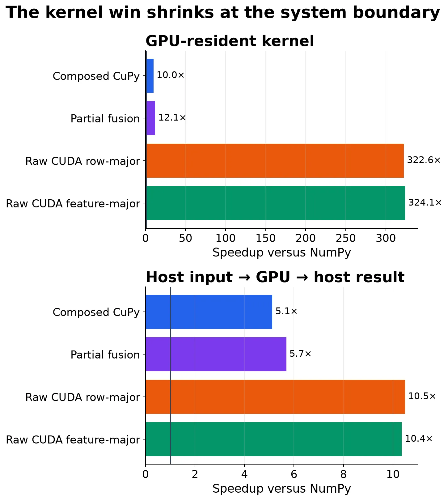
Composed CuPy was not a straw man. It delivered a useful fivefold one-shot win with much less code. Partial fusion bought another 11% by combining the standardize, clip, and weighting steps while leaving reduction and thresholding to CuPy. The raw kernel fused the entire row and nearly doubled the one-shot speedup again.
But the 324× number described a very specific contract: input already on the device, output left there, warm compiled kernel. Once the caller started and ended with NumPy arrays, roughly 97% of that ratio vanished.
The two ratios describe different systems: one with resident device data and one that starts and finishes in host memory.
The first crossover arrived at a few thousand rows
The 16-feature sweep started at 1,024 rows and doubled through 16,777,216. The one-shot paths behaved like this at four useful landmarks:
| Rows | Composed CuPy | Partial fusion | Raw row-major | Raw feature-major |
|---|---|---|---|---|
| 1,024 | 0.27× | 0.34× | 0.52× | 0.54× |
| 4,096 | 0.87× | 1.08× | 1.58× | 1.62× |
| 16,384 | 2.00× | 2.30× | 3.35× | 2.95× |
| 1,048,576 | 5.13× | 5.69× | 10.49× | 10.36× |
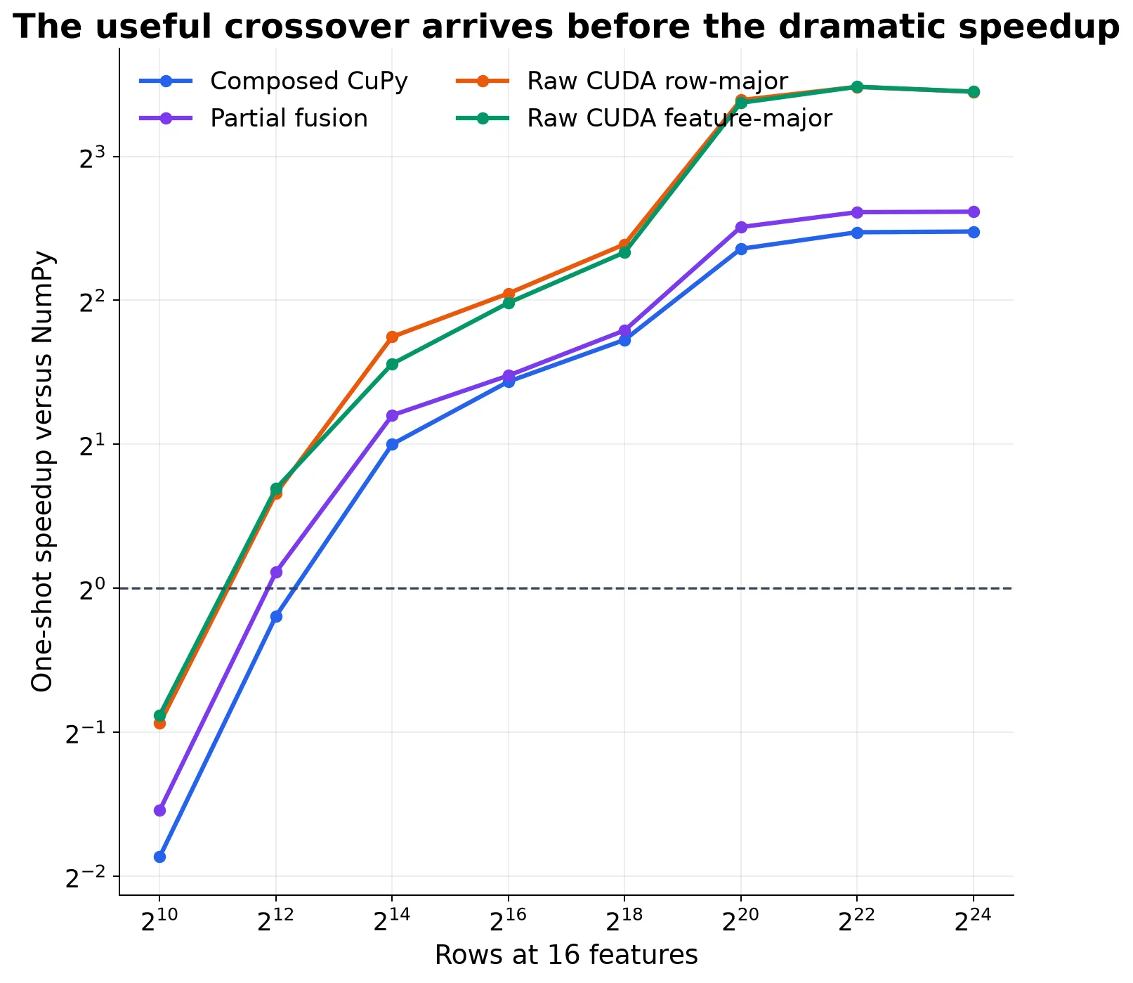
The raw kernels and partial fusion first beat NumPy at the tested 4,096-row point. Composed CuPy first won at 16,384. I would describe those as observed brackets, not exact crossover constants: the boundary lies between tested sizes and will move with CPU allocation, feature width, dtype, interconnect, library version, and upstream residency.
The first measured win was only 1.1–1.6×. Whether that latency saving justifies custom code, tests, packaging, and operational support depends on the application; a spectacular ratio is not required for a crossover.
Transfer bandwidth improved only with large copies
The copy calibration swept 4 KiB, 64 KiB, 1 MiB, 16 MiB, 256 MiB, and 1 GiB in both directions with pageable and CUDA-pinned host buffers. Buffer allocation was excluded.
At 4 KiB, every synchronized wall result remained below 0.5 GiB/s. At 1 GiB:
| Direction | Pageable | Pinned |
|---|---|---|
| Host to device | 15.09 GiB/s | 24.91 GiB/s |
| Device to host | 13.24 GiB/s | 20.44 GiB/s |
Pinned memory made the large copies materially faster, but “always pin” would still be incomplete advice. Registration or pinned allocation has its own cost, system memory is a shared resource, and tiny transfers remain dominated by fixed overhead. Reuse pinned buffers and move useful batches; do not turn a thousand tiny copies into a bandwidth benchmark by dividing bytes by time.
Feature-major layout cut the wide kernel to 0.661 ms
In the row-major kernel, one thread owns one row. During a given feature step, adjacent threads read values separated by the row width. In the feature-major kernel, adjacent threads read adjacent row values for that feature.
NVIDIA’s CUDA guidance treats coalescing as a high-priority optimization because a warp’s global-memory requests can otherwise require more memory transactions. The current programming guide describes the objective as maximizing the ratio of bytes used to bytes transferred in coalesced global-memory access.
The result depended on width. At 262,144 rows and 16 features, row-major and feature-major device timings were 0.041 and 0.052 ms. At 256 features they were 1.210 and 0.661 ms: feature-major was 1.83× faster. At 512 features it was about 1.86× faster.
The profiler supported that mechanism. For the 256-feature, 256-thread case, the row-major kernel reported 97.43 GB/s and 28.67% of peak DRAM throughput. Feature-major reached 306.89 GB/s and 90.32%. I do not use the instrumented durations as benchmark timings: Nsight Compute documents that selected metric sets can add collection overhead and replay work in its profiling guide.
The transpose changed the end-to-end calculation. Converting an already resident row-major array to a contiguous feature-major array took 2.967 ms at 262,144 × 256. The 0.549 ms kernel saving repaid that transpose after about 5.4 reuses. At 1,048,576 × 16, the layouts were so close that conversion required about 1,450 reuses. At 4,194,304 × 16 it required more than 10,000.
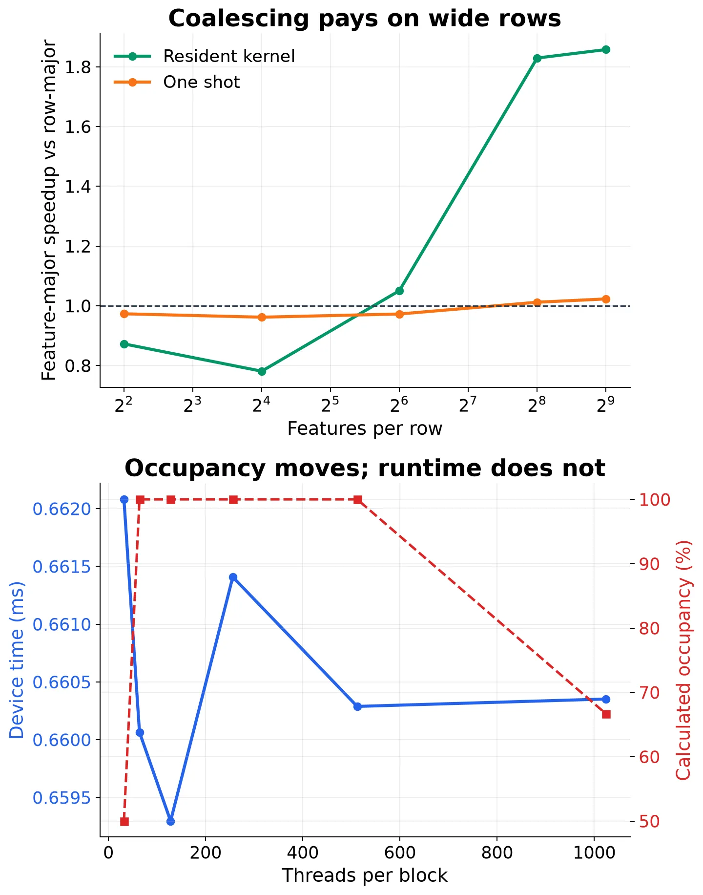
The one-shot comparison assumed the required host layout already existed and uploaded exactly one input array. Even then, feature-major only moved slightly ahead at 256 and 512 features because the upload and output path dominated the kernel saving. If an application begins with row-major data, it must add the conversion or negotiate feature-major layout with the upstream producer.
Coalesced access was clearly better for the wide resident kernel. Transposing every input to obtain it was not economical for the narrow cases.
Block size changed occupancy, not runtime
I padded each row to increase the stride between adjacent threads and retained blocks from 32 through 1,024 threads.
The padded-stride variant was up to about 16% slower than the ordinary row-major kernel at 4,194,304 × 16, depending on block size. At 262,144 × 256, it was nearly tied with row-major—both were already paying for the same broad non-coalesced access pattern. Making a bad layout slightly worse did not create a clean proportional penalty.
The block sweep was even more instructive. For feature-major 262,144 × 256:
| Threads per block | Calculated occupancy | Device time |
|---|---|---|
| 32 | 50.0% | 0.662 ms |
| 64 | 100.0% | 0.660 ms |
| 128 | 100.0% | 0.659 ms |
| 256 | 100.0% | 0.661 ms |
| 512 | 100.0% | 0.660 ms |
| 1,024 | 66.7% | 0.660 ms |
Calculated occupancy doubled from 32 to 64 threads. Runtime did not care. NVIDIA’s own best-practices guide says that higher occupancy does not always produce higher performance. Occupancy helps a kernel hide latency until some other limit takes over; it is not a score to maximize independently.
The controls narrowed the advice. Coalescing mattered on wide rows, padding hurt the narrow layout inconsistently, and every tested block size from 32 to 1,024 produced essentially the same wide feature-major runtime. A generic “256-thread blocks are best” rule would not describe these measurements.
Choosing the lowest level that earns its keep
Start with a NumPy reference and a composed CuPy implementation. The first protects correctness; the second establishes whether high-level GPU code is already sufficient. Composed CuPy delivered a 5.13× one-shot win at one million rows here without requiring raw CUDA.
Partial fusion is the next step when profiler or allocation evidence shows that intermediates and launches matter. It preserved a high-level reduction while improving one-shot time from 11.56 to 10.41 ms.
A raw kernel becomes reasonable when three conditions align:
- the operation is stable enough to carry custom correctness tests;
- enough compatible work can be fused to reduce memory traffic and launches; and
- data will stay resident or the batch is large enough to absorb its transfers.
Layout should be an upstream contract rather than a local afterthought. For wide, repeatedly reused inputs, feature-major data was clearly better. For narrow row-major inputs, a local transpose required so many reuses that the faster kernel was irrelevant.
Compile during initialization, retain CuPy’s cache between compatible runs, reuse transfer buffers, and batch small work. Cold compilation was tens of milliseconds; steady kernels were fractions of one.
Block tuning should follow measured time and inspection of registers and memory traffic. Occupancy alone did not predict the result.
These numbers do not cover irregular graphs, atomics under
contention, tensor-core matrix multiplication, unified-memory oversubscription,
multi-GPU communication, or C++ host extensions. The study used dense
synthetic float32 data, local memory, one GPU, warm steady execution, and a
single reduction-shaped operation.
For this operation, fusion removed launches and intermediate memory traffic; it could not remove host/device transfer or cold compilation (the same wall the full ML pipeline hit at larger scale). Coalescing helped when feature width exposed the memory pattern and when the layout was already available. Occupancy changed substantially without moving runtime. Those are the measurements I would want before accepting the maintenance cost of a custom kernel.
See what kernel fusion removes
Switch between separate passes and a fused pass. The output stays the same; the temporary matrix and extra global-memory trip disappear.