I Moved an Entire ML Pipeline to the GPU
fit() is an attractive place to stop a GPU benchmark.
It has a clean API boundary. It produces a large speedup number. And it leaves out most of the work required to make a model useful.
My actual question was less convenient:
When does classical machine learning become worth moving to a GPU after preprocessing, feature engineering, transfers, training, inference, and the final host-visible answer are all charged to the same decision?
This is the practical question behind fraud and anomaly scoring, customer propensity models, segmentation, forecasting features, and other classical ML systems that still do useful work without a giant neural network. Training may run nightly on a large table while inference arrives in tiny online batches. Moving only the estimator can improve a benchmark and leave the application unchanged—or slower.
I ran two related studies on an RTX PRO 4000 Blackwell SFF with 24 GB of
VRAM. The first compared CPU libraries, unchanged supported APIs under
cuml.accel, and native GPU implementations across seven estimators. The
second built one complete dense-numeric pipeline and deliberately changed
where its data lived.
The largest estimator result was a 67.2× one-shot UMAP win. The complete
pipeline gave a less spectacular and more applicable comparison. At one million
rows, the GPU-resident path was 4.74× faster end to end. The unchanged
cuml.accel path reached 2.10×, while an intentional GPU-to-CPU-to-GPU island
still reached 3.13×.
At 5,000 rows, cuml.accel was only 1.02×—well inside the replication ranges.
Native residency was 1.25× faster, but it saved about three milliseconds. At a
fixed 100,000 rows, widening the input from 16 to 256 features moved the
GPU-resident win from 1.97× to 6.15×.
Those timings show how much an impressive fit result can depend on the work surrounding it and where that work executes.
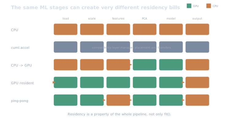
The estimator is one box in a longer path. The placement topology determines how often the data crosses the device boundary.
Two studies: estimator and application
The estimator matrix covered PCA, KMeans, Logistic Regression, Random Forest, UMAP, HDBSCAN, and XGBoost. It varied row count from 20,000 to five million, feature width from 16 to 1,024, inference batch size from one to 65,536, and included a separate well-separated manifold lane for meaningful UMAP and HDBSCAN quality checks.
Each supported condition compared:
- the CPU implementation from scikit-learn,
umap-learn,hdbscan, or XGBoost; - the same scikit-learn-style API under
cuml.accel; and - native cuML with an explicit host-to-device upload.
XGBoost used its CPU and native CUDA paths; it is not a cuml.accel estimator.
The native path followed XGBoost’s current GPU interface: device="cuda" with
the histogram tree method, as documented in the
XGBoost GPU guide.
I timed input loading, explicit upload, model fitting, batched inference, and host materialization separately. “One-shot fit” means warm-cache loading plus explicit transfer plus fit. It is still smaller than an application, but it prevents a fast kernel from receiving credit for a free upload.
The pipeline matrix then measured this complete path:
load -> standardize -> nonlinear features -> PCA -> logistic regression -> probability inference -> host materializationFive placements made the residency cost visible:
| Placement | What moved |
|---|---|
| CPU | Nothing; NumPy and scikit-learn throughout |
cuml.accel | Unchanged APIs; transfers managed behind the compatibility layer |
| GPU resident | One upload; CuPy and cuML through the final materialization |
| CPU to GPU | CPU preprocessing, then one transition for PCA and the model |
| Ping-pong | GPU scaling, a CPU feature island, then GPU model stages |
The last topology is intentionally awkward. It represents the real pipeline where one unsupported transformation is enough to interrupt device residency.
Equivalent models did not need identical internals
CPU and GPU implementations need not produce identical coefficients, principal-component signs, tree structures, or cluster labels. Demanding that would test implementation identity, not useful equivalence.
Instead, every performance result had to pass an algorithm-appropriate quality gate:
- retained explained variance for PCA;
- adjusted Rand score for KMeans and HDBSCAN;
- trustworthiness for UMAP; and
- ROC AUC, log loss, and accuracy for the classifiers.
The cuml.accel logs also had to say that execution ran on the GPU. Any CPU
fallback invalidated the matrix. That matters because RAPIDS documents that
support can depend on estimator, method, parameters, and input,
not merely the imported class name. Its
logging tools
are part of a benchmark’s evidence, not optional debugging decoration.
Every condition ran in a fresh process pinned to eight CPU threads. One
unmeasured warmup preceded three measured trials, and publication values are
medians across three independent replications. GPU work was synchronized at
timing boundaries. Inputs were deterministic float32 arrays read from a warm
operating-system cache.
The harness sampled GPU memory, utilization, and device power. I publish its device-energy estimate as diagnostic evidence, but I do not use it to claim a whole-system energy win: CPU package power, DRAM, storage, and power-supply losses were outside the measurement boundary.
The complete public companion in
ramwise-examples
contains the output-complete notebook, derived results with replication ranges,
quality evidence, tested harness, publication matrices, digest-pinned
container, and exact package specification.
Fit time overstated several wins
The largest one-shot estimator win was native UMAP at 100,000 rows and 16
features: 67.2× faster than CPU. The cuml.accel path reached 65.7× in the
same condition. At one million rows and 64 features, accelerated Random Forest
was 24.8× faster one shot; native cuML reached 22.8×.
Those are the clean wins. PCA showed why the second timer mattered.
At 100,000 rows and 1,024 features, native PCA made fit() 43.4× faster.
Warm-cache loading and the explicit upload reduced the one-shot win to
7.17×. Native Logistic Regression in that same wide condition made the fit
1.54× faster but lost one shot at 0.87× CPU speed. At 20,000 rows and 64
features, both Logistic Regression GPU paths were about 0.52× CPU speed.
Across all tested conditions, median fit and one-shot speedups told the same story at different volumes:
- native PCA: 18.7× fit, 3.57× one shot;
- native KMeans: 16.1× fit, 5.58× one shot;
- native Logistic Regression: 1.95× fit, 1.07× one shot;
- GPU XGBoost: 3.86× fit, 3.73× one shot; and
cuml.accelRandom Forest: 9.50× fit, 9.44× one shot.
UMAP and Random Forest spent enough time in the estimator that loading barely changed the conclusion. PCA and KMeans exposed the upload tax. Logistic Regression sat close enough to the boundary that row count and width could change the winner.
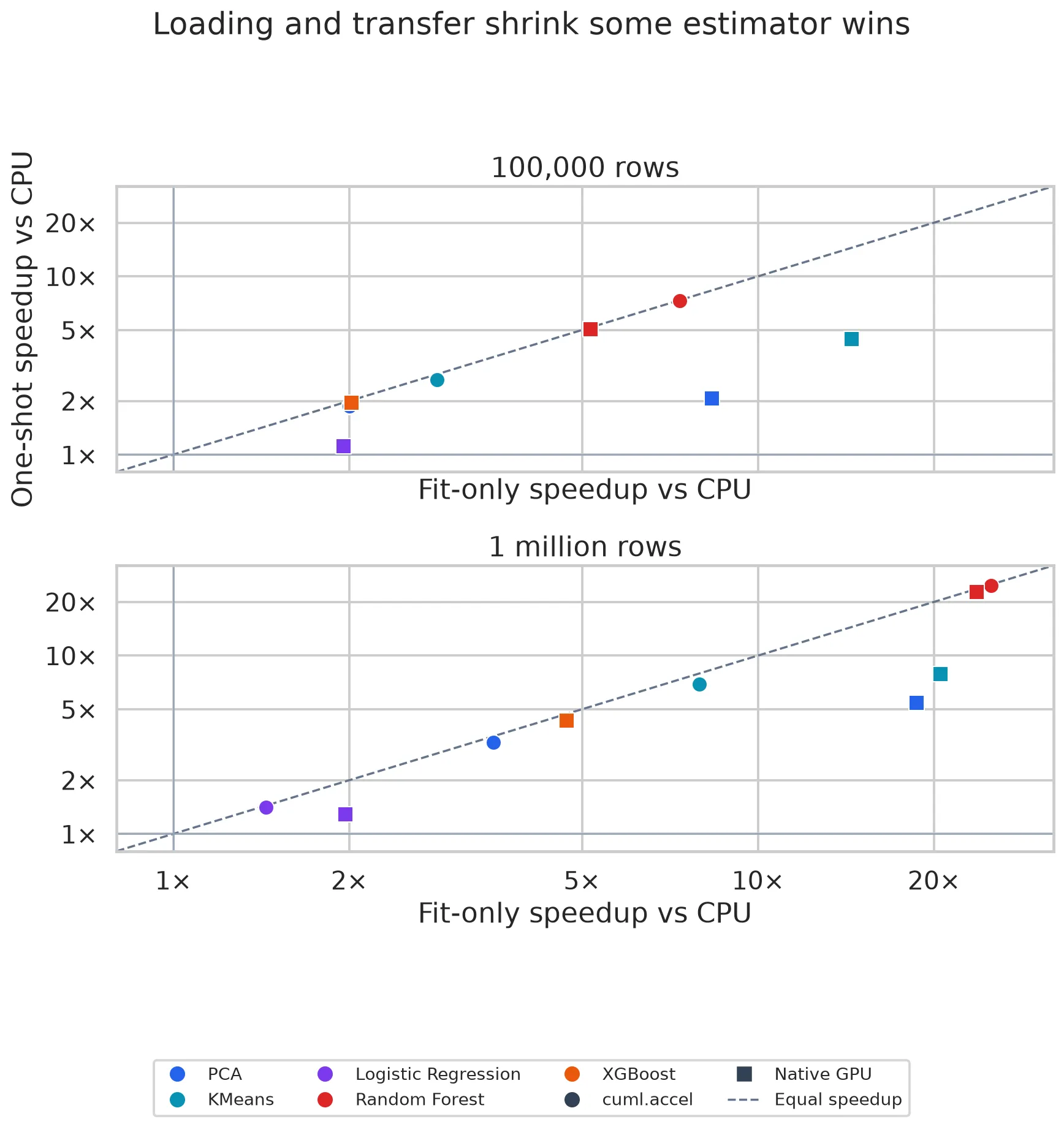
A library microbenchmark and an application estimate answer different questions. The fit-only value describes a reused, resident workload. The one-shot value describes a model trained once from a host-resident input.
RAPIDS makes the same qualitative warning in its own
cuml.accel benchmark guidance:
larger problems generally benefit more, transfer overhead can dominate small
ones, and native GPU-resident data can avoid conversion costs. The useful
addition from this experiment is a controlled measurement of that warning on
this workstation and these algorithms.
One transfer each way was the fastest topology
The 5,000-row result was a useful warning about ratios. CPU took 15.40 ms. The
GPU-resident pipeline took 12.36 ms, a 1.25× speedup with non-overlapping
replication ranges—but only a three-millisecond saving. The cuml.accel path
took 15.13 ms, and its range overlapped CPU. Calling either result an economic
crossover without discussing engineering cost would be theatre.
At 20,000 rows, GPU residency reached 1.85× and the forced CPU island reached 1.43×. At 100,000 rows, those became 2.82× and 1.68×. At one million rows, the complete timings were:
- CPU: 1.904 seconds;
cuml.accel: 0.905 seconds, or 2.10×;- GPU resident: 0.402 seconds, or 4.74×;
- CPU preprocessing followed by GPU: 0.613 seconds, or 3.10×; and
- GPU scaling, CPU features, then GPU models: 0.609 seconds, or 3.13×.
Feature width strengthened the result even without more rows. At 100,000 rows, GPU residency was 1.97× faster with 16 input features, 2.82× with 64, and 6.15× with 256. The wider CPU PCA had more work to lose.
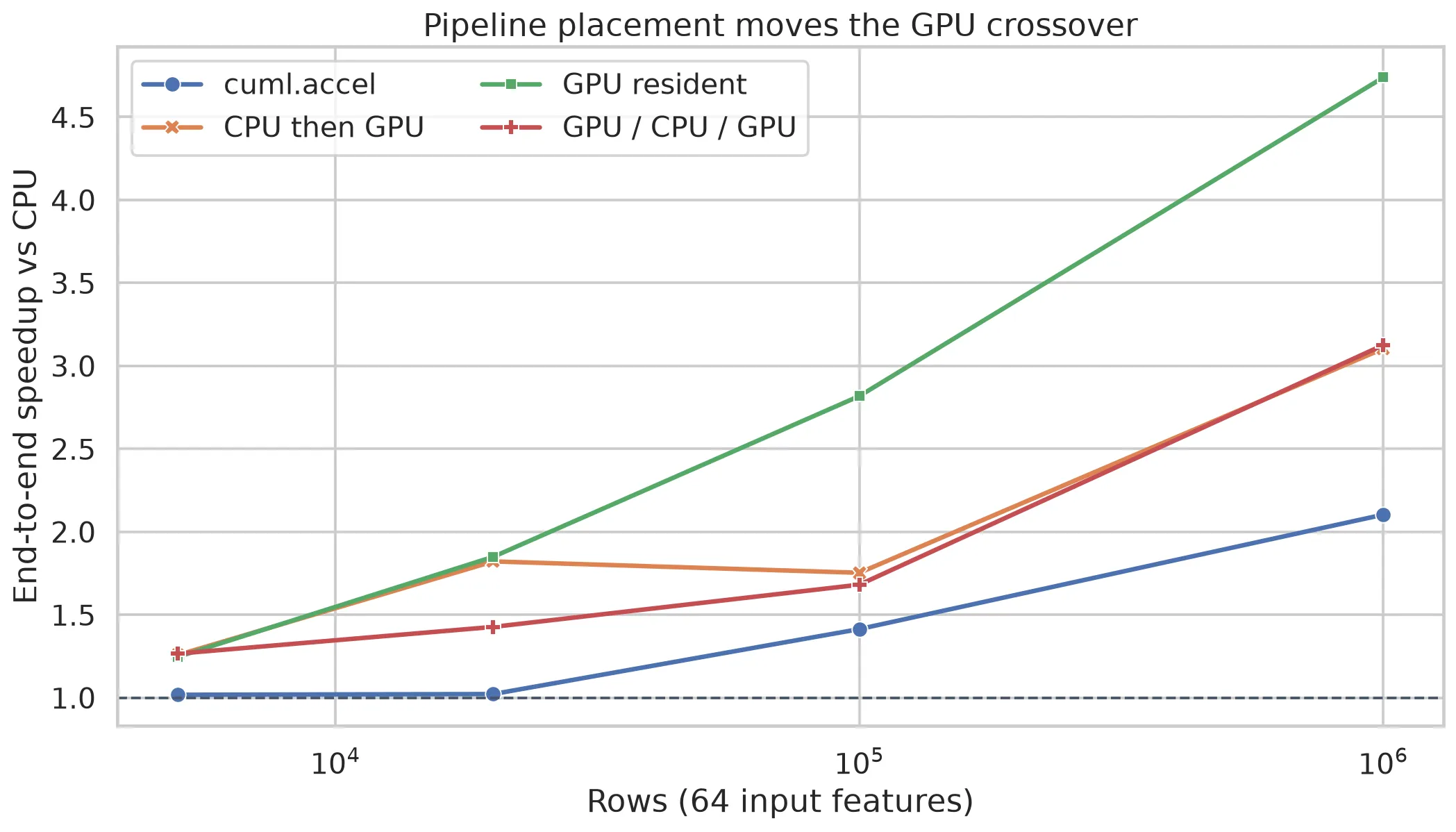
The fastest path crossed once in each direction: one grouped upload near the start and one final materialization. At one million rows it moved about 0.241 GiB to the device and 0.003 GiB back.
The ping-pong path recorded four directional boundary events and moved about 0.525 GiB to the GPU plus 0.241 GiB back. It was 51% slower than the resident path. Yet it still beat CPU by 3.13× because the accelerated scaling, PCA, and model stages were large enough to pay the transfer bill. At this scale it was effectively tied with the CPU-then-GPU topology; GPU scaling recovered about what the extra round trip spent.
At 100,000 rows, the same CPU island cut the resident speedup from 2.82× to 1.68×. Placement cost was not a fixed penalty. It competed with the amount of accelerated work on either side.
A CPU island had a concrete price: materialize, cross PCIe, do the host work, upload again, and reconstruct the GPU execution context around it. The larger GPU stages in this matrix repaid that price; smaller ones did not.
This is also why “drop-in” and “GPU resident” are different product promises.
cuml.accel is valuable because it lowers migration cost and can expose
unsupported paths through logging. Native CuPy/cuML code gives the application
more control over residency. The first optimizes engineering effort; the
second can optimize the data path. Which matters more depends on the workload.
Small-batch inference often stayed on the CPU
At the one-million-row condition and 64 features, native GPU inference on a single row was slower than CPU for KMeans, Logistic Regression, PCA, and XGBoost. The speedups were 0.31×, 0.22×, 0.42×, and 0.22× respectively. Random Forest was the exception: both GPU paths beat CPU even at batch one, with native cuML at 65.8×.
At a 65,536-row batch the native path crossed over for every one of those
models: 3.48× for KMeans, 1.77× for Logistic Regression, 1.88× for PCA, 40.1×
for Random Forest, and 5.93× for XGBoost. The unchanged cuml.accel API still
lost that large-batch inference comparison for KMeans, Logistic Regression,
and PCA, even though it had accelerated their fits.
Training acceleration therefore did not imply serving acceleration. The estimator, batch, output contract, and residency still had to agree.
For an online service, a one-row request is not a 65,536-row batch divided by 65,536. Launch overhead, conversion, queueing, and materialization do not scale that way. The published table therefore keeps measured batch latency and throughput separate and derives a reuse count only when the candidate’s repeated inference is actually faster than CPU.
That count is a planning aid, not a serving SLA. This experiment did not model concurrent clients, dynamic batching, model loading, network latency, or tail percentiles.
A migration path from scikit-learn
cuml.accel is a sensible first probe for a supported scikit-learn workflow.
The environment should be pinned, dispatch logging enabled, fallback rejected
in performance tests, and the complete call path timed. On this pipeline its
median savings were only 0.27 and 0.57 milliseconds at 5,000 and 20,000 rows.
The advantage reached 1.41× at 100,000 rows and 2.10× at one million.
Native CuPy/cuML becomes easier to justify when a pipeline is wide, reused, or already produces device-resident data. Here that extra code delivered 4.74× rather than 2.10× at one million rows, and 6.15× at 100,000 rows with 256 features.
Latency-sensitive, tiny-batch inference should remain on the CPU unless its specific estimator proves otherwise. Native PCA, KMeans, Logistic Regression, and XGBoost all lost at batch one after training on one million rows. Random Forest was the exception; the other four crossed at the tested 65,536-row batch.
For mixed pipelines, bytes and materializations are more informative than a count of “GPU steps.” A material CPU island can be fused, reimplemented, or surrounded by enough compatible GPU work to amortize the crossings. Otherwise, keeping the pipeline on the CPU may be the simpler choice.
These are measured intervals rather than universal thresholds. They cover dense numeric arrays, warm local input, fixed algorithms, one workstation, and data that fits in VRAM. Sparse text, categorical-native workflows, hyperparameter search, distributed training, cold storage, and production serving queues can move every crossover reported here.
Estimator compatibility also belongs in the performance test. Support can vary with method and parameters, and a later library version may dispatch differently. Pinning packages and asserting the GPU log is stronger evidence than observing that a run appeared to use the device.
The transfer-once topology is also what the hand-written CUDA kernels rewarded: the kernel was fast, and the copies around it decided the result.
Taken together, the measurements favor moving a complete compatible interval
to the GPU—not merely replacing fit(). More rows, wider features, expensive
estimators, larger inference batches, and model reuse all lengthen that interval
or make it more valuable.