The Radio Won't Wait for Your FFT
Most benchmarks are patient. A radio is not.
If one block arrives every four milliseconds, the previous block has four milliseconds to clear the pipeline. A six-millisecond FFT is not merely slow. It creates two milliseconds of debt. Repeat that long enough and a bounded receiver buffer has only one possible answer: discard samples.
That failure mode matters in software-defined radio receivers, spectrum monitors, wireless gateways, radar and sonar processing, and any sensor stream that cannot ask its source to pause. Once processing falls behind acquisition, the system must grow a queue, increase latency, or lose part of the signal.
That changed the question I wanted to measure. I was not looking for the largest GPU speedup over an isolated FFT. I wanted to know when a complete signal-processing path stopped keeping up with its source.
I replayed deterministic complex I/Q blocks through a 129-tap filter, windowing, 2,048-point FFTs, power spectra, and a detector. A schedule-driven producer fed an eight-block queue without waiting for the consumer. I compared an eight-core NumPy/SciPy path with three CuPy placements: pageable host input, pinned host input, and input already resident on the GPU.
The longer confirmation made the boundary hard to miss. With 131,072 samples per block, the CPU had no deadline misses or drops at 20 million samples/s. At 30 million it missed every deadline and dropped 1.05% of arrivals. The pinned GPU had a 0.079% miss rate and no drops at 300 million samples/s. At 450 million, it missed 52.5% of deadlines.
The GPU moved the usable range by roughly an order of magnitude. It did not turn a general-purpose Ubuntu process into a hard-real-time system.
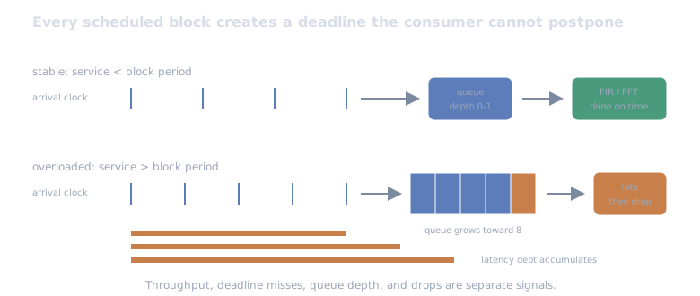
The queue converts a small service-time deficit into rising latency and, eventually, missing samples. That is why throughput alone is not the SLA.
The queue was the benchmark
The pipeline for one block was:
complex64 I/Q + FIR history -> 129-tap frequency-domain convolution -> non-overlapping 2,048-sample frames -> Hann window -> batched FFT -> power spectrum -> peak-to-mean detector -> host-visible peak bin and decisionBlocks alternated between a strong injected tone and noise. Every fresh process first ran the SciPy reference and compared GPU peak bins, peak-to-mean ratios, and detector decisions. The tone had to be found in every frame; the noise-only control had to produce no detections. A performance row was written only after those checks passed.
The old cuSignal package is not part of this stack. RAPIDS archived the
cuSignal repository after its 23.08
release and moved much of the work into CuPy. The current implementation uses
cupyx.scipy.signal
and cupy.fft.
There were two kinds of run.
The capacity pass processed blocks back to back. It answered, “How many samples per second can this implementation service when it never waits?” The paced pass answered the less comfortable question: “What happens when blocks arrive on their own clock?”
For the paced run:
block period = samples in block / incoming sample rate
deadline miss: completion time > scheduled arrival + block perioddrop:          a new arrival finds the eight-block queue full
The producer never applied backpressure. That is important. A benchmark that waits for its consumer silently converts an overloaded radio into a slower radio.
I kept capacity and latency separate
The full exploratory matrix had 192 fresh-process jobs. It covered 8,192, 32,768, 131,072, and 524,288 samples per block for capacity, then paced 8K, 32K, and 131K blocks across rates selected around the measured CPU and GPU limits. Every condition had three independent replications in seeded random order.
A second matrix repeated 12 boundary conditions for five seconds each, again in three fresh processes. That longer confirmation is the source of the deadline and drop claims in this article.
The machine was the RTX PRO 4000 Blackwell SFF with 24 GB of VRAM. The Ubuntu 26.04 host kept its usual services running. The benchmark container was Ubuntu 24.04 with Python 3.12, NumPy 2.4.6, SciPy 1.16.3, CuPy 14.1.1, and CUDA 13.1. The container was pinned to CPU cores 0-7.
Capacity used three unmeasured warmups, seven measured trials of 16 blocks, and three replications. GPU wall timing ended only after stream synchronization. CUDA events separately measured upload, device work, and the small result download. Warmups also kept one-time FFT planning out of the steady-state result; CuPy documents that its FFT plan cache is enabled by default, while cuFFT documents both reusable plans and batched transforms.
Batching changed the machine
The capacity result was not one GPU number:
| Samples/block | CPU | GPU pageable | GPU pinned | GPU resident | Pinned/CPU |
|---|---|---|---|---|---|
| 8,192 | 22.1 MS/s | 30.2 MS/s | 30.5 MS/s | 31.1 MS/s | 1.38x |
| 32,768 | 31.9 MS/s | 110.6 MS/s | 116.1 MS/s | 122.1 MS/s | 3.65x |
| 131,072 | 29.6 MS/s | 417.8 MS/s | 498.3 MS/s | 513.9 MS/s | 16.84x |
| 524,288 | 32.1 MS/s | 1,007.4 MS/s | 1,443.1 MS/s | 1,999.7 MS/s | 44.93x |
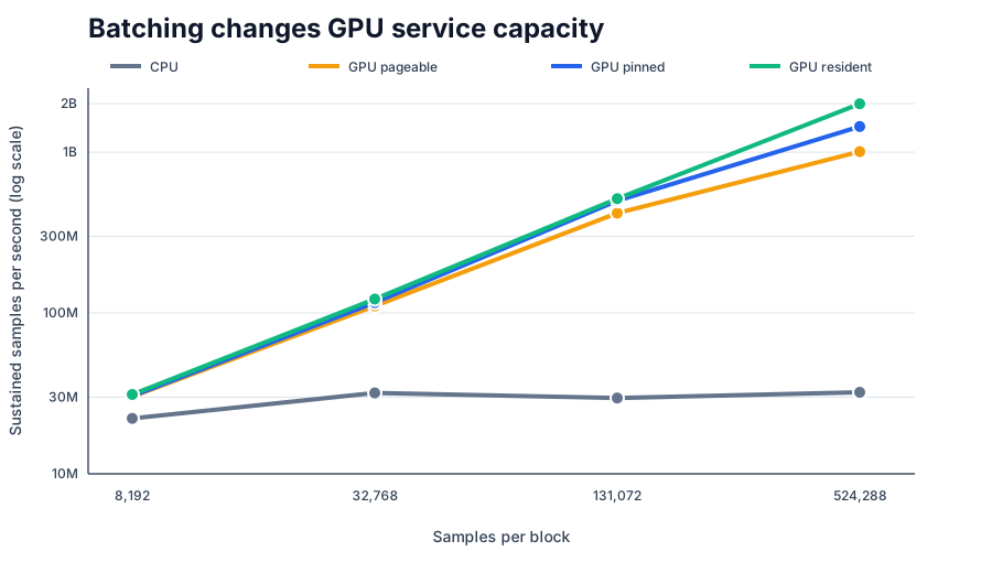
The CPU flattened near 30 million samples/s after the smallest block. The GPU kept finding more parallel work. At 8K samples, fixed launch, synchronization, and result costs left only a 1.38x pinned-GPU win. At 524K, the same placement was 44.9x faster.
That 1.44 billion-sample/s row is a service-capacity measurement, not an SDR claim. The block is large, the data is synthetic, and the pipeline does not include radio ingress. The resident 2.00 billion-sample/s result is an even narrower upper bound: no host upload at all.
Block size is also latency. At 20 million samples/s, merely collecting an 8K block takes 0.410 ms; collecting a 131K block takes 6.554 ms. The paced timer starts when a complete block is ready. A sample near the front of that block has already waited almost one block period before processing begins.
Larger batches make the GPU look better and give the scheduler more absolute slack. They also make the oldest sample older. A real design has to choose all three together: sample rate, block size, and allowed end-to-end latency.
At 30 million samples/s, the CPU queue filled
The 131K five-second confirmation looked like this:
| Path | Input rate | Block period | Median service | p99 latency | Misses | Drops |
|---|---|---|---|---|---|---|
| CPU | 20 MS/s | 6.554 ms | 4.688 ms | 5.591 ms | 0% | 0% |
| CPU | 30 MS/s | 4.369 ms | 4.407 ms | 41.615 ms | 100% | 1.05% |
| CPU | 40 MS/s | 3.277 ms | 4.332 ms | 42.370 ms | 100% | 25.16% |
| GPU pinned | 100 MS/s | 1.311 ms | 0.432 ms | 0.817 ms | 0% | 0% |
| GPU pinned | 300 MS/s | 0.437 ms | 0.268 ms | 0.340 ms | 0.079% | 0% |
| GPU pinned | 450 MS/s | 0.291 ms | 0.259 ms | 0.331 ms | 52.51% | 0% |
At 40 million samples/s, the CPU processed roughly three quarters of the offered rate and discarded one arrival in four. That is the uncomplicated overload case: median service was slower than the arrival period, so the debt could only grow.
The 30-million case was closer and more revealing. Median service was 4.407 ms against a 4.369 ms period. The deficit was only 0.9%, but the eight-block queue filled, median latency reached 37 ms, and drops appeared during the longer run. Near parity, a small service deficit does not stay small. It accumulates.
The 32K block told the same story sooner. CPU was clean at the tested 20 million samples/s point, missed 44.3% of deadlines at 30 million, and dropped 18.9% at 40 million. The pinned GPU stayed below 0.3% misses at 80 million and missed 50.5% at 110 million.
I would state these as tested brackets, not exact crossovers. CPU failure lies between 20 and 30 million samples/s for these two useful block sizes and this stack. The pinned GPU’s low-miss boundary lies between 80 and 110 million for 32K blocks, and between 300 and 450 million for 131K blocks.
Throughput headroom did not guarantee a deadline
The 450-million pinned-GPU result is the useful catch.
Its median service time was 0.259 ms. The block period was 0.291 ms. Dividing one by the other says the consumer had about 12% median throughput headroom. Yet 52.5% of blocks were late, because median arrival-to-completion latency was 0.295 ms and p99 was 0.331 ms.
The 32K CPU case at 30 million samples/s did the same thing at a larger scale: median service suggested 13% headroom, but 44.3% of deadlines were missed.
Service capacity answers whether an infinite stream is stable in the long run. A per-block deadline also pays wake-up delay, interpreter and scheduler jitter, queue position, and synchronization. A stable queue can still deliver late answers. Conversely, a one-second run can look stable just before a tiny service deficit becomes a drop; that is why I added the five-second confirmation.
This was a normal Ubuntu kernel and an ordinary Python process. Canonical’s
Real-time Ubuntu documentation
describes the PREEMPT_RT kernel, priority scheduling, IRQ tuning, and CPU
isolation needed for more deterministic response. It also recommends measuring
maximum latency under representative load with tools such as
cyclictest.
The experiment measures soft-real-time behavior. It does not certify a hard deadline.
Pinned memory helped only after blocks became worth moving
At 8K samples, pinned and pageable GPU capacity differed by less than 1%. At 32K, pinned was 5% faster. The gap grew to 19% at 131K and 43% at 524K.
The pinned path deserves a precise contract. I allocated page-locked replay buffers and populated them before timing. That represents an acquisition stack that can DMA directly into reusable pinned buffers. If an application first receives a pageable array and then copies it into pinned memory, it owes that extra host copy; an earlier pilot did exactly that and erased the benefit.
NVIDIA’s CUDA best-practices guide recommends pinned memory for higher transfer bandwidth and requires it for asynchronous host/device copies. The same guide warns that pinned memory is a scarce system resource and that allocation or registration is heavyweight. That matches this result: preallocate a small buffer pool and reuse it. Do not pin everything by reflex.
This harness used one non-default stream and processed one block at a time. Copy and compute were ordered within that stream. A production implementation could double-buffer across streams and overlap the next upload with current compute on hardware that supports concurrent copy and execution. The NVIDIA guide documents that pattern. It is a reasonable next optimization, not free performance I credited to this result.
The resident path shows why the rest of the pipeline matters. At 131K, resident input was only 3% faster than pinned. At 524K it was 39% faster. If channelization, beamforming, inference, or recording also runs on the GPU, keeping intermediates there can avoid paying the bus again. If the detector’s full spectrum immediately returns to a CPU, this experiment’s tiny host-visible output is too optimistic.
What this result changes for me
I would make the queue part of every streaming accelerator benchmark.
A back-to-back timing loop is still useful. It locates service capacity and separates transfer from device work. But it cannot show the point where latency debt fills a real buffer. The producer has to keep its own clock, the queue has to be bounded, and misses and drops have to be first-class results.
For a live system, I would also require:
- the real SDR or capture device, including driver and packet behavior;
- a measured choice between pageable, directly pinned, and device-resident buffers;
- block-fill time in the end-to-end latency budget;
- a longer soak under representative host load;
- an explicit loss policy when the queue fills; and
- PREEMPT_RT, scheduler, affinity, and IRQ experiments if deadlines are strict.
I did not measure overlapping FFT windows, multi-channel input, SDR ingress, energy, thermal throttling during a long soak, or hard-real-time Linux. Those are limits, not footnotes.
The public companion in
ramwise-examples
contains the self-contained output notebook and all three derived evidence
tables: capacity, the full paced exploration, and the five-second boundary
confirmation. The notebook runs its CPU example without CUDA and enables the
CuPy path when a compatible GPU is present.
The GPU speedup was not the most useful finding. The queue was.
Once the CPU’s sustained service rate fell below the radio’s arrival rate, acceleration stopped being a throughput luxury. Missing data changed the answer. But the GPU boundary supplied the final warning too: even when median throughput said there was room, a general-purpose scheduler could still make a block late.
The radio will not wait for the average.
The video version of this test used the same deadline-first method with hardware encode and decode engines in the path.
Watch the FFT reveal the signal
Move two tones through noise and watch their peaks appear in the live spectrum and waterfall.