How Much of a Spark Plan Actually Runs on the GPU?
I wanted to know how much of a Spark plan had to stay on the GPU before partial acceleration stopped being useful.
That is the migration problem for a mature Spark estate. A production ETL job may be mostly supported scans, joins, and aggregates but still contain a Python UDF for redaction, business rules, feature scoring, or a library call that has no GPU equivalent. The plugin can accelerate the supported operators, yet the rows on either side of that CPU-only island still have to move somewhere.
I built one ETL job, ran it with ordinary PySpark and with the RAPIDS Accelerator, and then damaged the GPU plan on purpose. I inserted vectorized Python UDFs after aggregation, after filtering, before filtering, and in two separated locations. I widened one of those CPU islands from one input column to twelve. Then I inspected the executed physical plan and measured the mixed plan against the equivalent CPU plan.
The native GPU plan did win at fifty million rows. A CPU island after aggregation preserved most of that win. Moving the same one-column UDF before the selective filter erased it. Two separated CPU islands were worse still: the hybrid plan took 2.559 seconds against 1.921 seconds for CPU-only.
That is 33% slower than staying on the CPU.
Fallback did not impose one fixed penalty. Its cost followed the position of the CPU work, the amount of data reaching it, and whether the plan had to cross back to the GPU afterward.
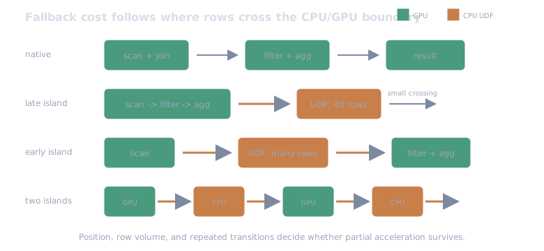
A CPU island is not just one slow operator. Its position determines how many rows cross the boundary, and another GPU stage determines whether they must cross back.
The ETL was ordinary on purpose
The fact table was deterministic, wide, and stored as Zstandard Parquet. It contained identifiers, order measures, short strings, free text, and twelve floating-point metrics. A 100,000-row customer dimension supplied segment, region, and risk.
The query did the sort of work I would expect in an analytical pipeline:
Parquet scan → filter amount and quantity → broadcast customer join → derive net amount → group by region and segment → count, sum, and average → sort the 40-row resultBoth modes used Spark 3.5.8, Java 17, and RAPIDS Accelerator 26.06.1 in the
same digest-pinned CUDA 13 container. CPU mode still loaded the plugin; only
spark.rapids.sql.enabled changed. The host was Ubuntu 26.04 with an NVIDIA
RTX PRO 4000 Blackwell SFF (24 GB), an Intel Core Ultra 9 285HX, and 122 GiB
of RAM. Spark ran in local[16] with 32 shuffle partitions.
That last detail is a boundary on the claim. NVIDIA describes local mode as a development and testing setup, not a production deployment. This experiment isolates physical-plan behavior on one GPU; it does not reproduce a cluster, remote object storage, network shuffle, or scheduler economics. See NVIDIA’s local-mode guidance.
Each condition ran in a newly started JVM, performed one warmup, then two
measured actions. I repeated each condition in three process-level
replications and randomized their order. The timer covered collect() through
the final CPU-backed rows, but not JVM startup. Every result matched a per-size
CPU reference.
The public companion in
ramwise-examples
contains all 78 process-level rows, the output-complete notebook, the exact
matrices, the tested harness, checksums, the Python dependency lock, and the
methodology. Raw event logs and private machine paths remain in the internal
lab.
Establishing the all-GPU baseline
Before introducing fallback, I needed to know whether the fully supported GPU plan had enough work to pay for itself.
| Fact rows | CPU | GPU | CPU / GPU |
|---|---|---|---|
| 1 million | 0.308 s | 0.368 s | 0.84× |
| 5 million | 0.330 s | 0.428 s | 0.77× |
| 10 million | 0.374 s | 0.439 s | 0.85× |
| 20 million | 0.480 s | 0.455 s | 1.05× |
| 50 million | 0.587 s | 0.514 s | 1.14× |
The CPU won through ten million rows. The GPU reached practical parity at twenty million and led by 1.14× at fifty million.
I would not turn those five points into a universal crossover rule. They are warm-cache local-NVMe action timings on one strong workstation CPU. They do establish something important for the next test, though: at fifty million rows the native GPU plan had a real but modest advantage available to lose.
Making the CPU islands visible
A scalar Pandas UDF is still Python work. Current RAPIDS can partially
accelerate the ArrowEvalPythonExec backend—the transfer between the JVM and
Python—and can schedule GPU resources for Python, but that does not magically
turn arbitrary Python code into a GPU kernel. NVIDIA’s
operator documentation
makes that distinction explicit.
For the main fallback matrix, I set:
spark.rapids.sql.exec.ArrowEvalPythonExec=falseThat deliberately made every Pandas UDF a visible CPU island. It is a stress test of unsupported-plan fragmentation, not a claim about the default setting in RAPIDS 26.06.1.
The representative mixed plan looked like this:
GpuFileSourceScan → GpuColumnarToRow → ArrowEvalPython (CPU) → GpuRowToColumnar → GpuFilter → GpuBroadcastHashJoin → GpuHashAggregate → GpuSort → final host collectionThe native GPU plan already had its final host transition because the result was collected into Python. One deliberate CPU island produced three transition lines in the executed plan. Two separated islands produced five.
This is why I inspected the executed plan rather than trusting the
configuration. NVIDIA recommends spark.rapids.sql.explain for exactly this
gap analysis, and its Qualification tools report unsupported operators,
unsupported expressions, and transition counts. The official
workload qualification guidance
also makes the right nuanced point: a query can still benefit when some work
falls back; it depends on how critical the CPU portion is.
The same UDF cost more before the filter
The fallback matrix fixed the fact table at fifty million rows. The timings below are medians across the three process-level replication medians. A ratio above 1.0 means the hybrid GPU plan won against the equivalent CPU plan.
| Plan topology | CPU | Hybrid GPU | CPU / GPU | GPU transition lines |
|---|---|---|---|---|
| Native | 0.626 s | 0.511 s | 1.22× | 1 |
| UDF after aggregation | 0.940 s | 0.788 s | 1.19× | 3 |
| UDF after filtering | 1.166 s | 1.113 s | 1.05× | 3 |
| UDF before filtering | 1.326 s | 1.351 s | 0.98× | 3 |
| Two separated CPU islands | 1.921 s | 2.559 s | 0.75× | 5 |
The late UDF touched only the forty aggregate rows. Crossing into Python was still overhead, but almost all of the expensive scan, filter, join, and aggregation remained useful GPU work. The hybrid plan retained a 1.19× lead.
Putting the same one-column identity UDF after the filter left the GPU with a 1.05× lead—practical parity at these sub-second-to-one-second runtimes. Moving it before the selective filter made the CPU and GPU plans effectively tie. The plan crossed the boundary before Spark had reduced the data.
Then I split the unsupported work into two islands, with GPU work between them. That forced the plan to leave columnar GPU execution, return, leave again, and return again before final collection. The hybrid plan was only 0.75× as fast as CPU-only, or about 33% slower in elapsed time.
The failing pattern was a fragmented plan with repeated crossings around meaningful amounts of data, not the mere presence of one unsupported operator.
Wider fallback did not steadily get worse
I also widened the single pre-filter UDF so that it consumed 1, 4, 8, and 12 numeric columns.
| Columns entering one CPU island | CPU | Hybrid GPU | CPU / GPU |
|---|---|---|---|
| 1 | 1.326 s | 1.351 s | 0.98× |
| 4 | 2.022 s | 1.836 s | 1.10× |
| 8 | 2.767 s | 2.595 s | 1.07× |
| 12 | 3.847 s | 3.343 s | 1.15× |
The wider UDF slowed both modes. Surprisingly, the hybrid plan again beat its CPU equivalent at widths four, eight, and twelve. Width alone did not produce a monotonic GPU penalty.
This is also why the comparison baseline matters. If I compared every hybrid case only with the 0.626-second native CPU plan, I could make every UDF look like a GPU failure. That would confuse the cost of executing the Python logic with the incremental cost of crossing the device boundary. The fair question is whether the mixed plan beats the same logical plan run entirely on CPU.
The evidence supports “placement and repeated boundaries mattered more than width for this workload.” It does not support a formula such as “N columns of fallback make a GPU uneconomic.”
Why I excluded the default-bridge timings
Because the main matrix disables a feature that is enabled by default, I ran a
separate diagnostic with RAPIDS’ accelerated Python columnar bridge restored.
The executed plan correctly reported that ArrowEvalPythonExec would
partially run on the GPU while the Python expression remained Python.
I am not publishing its timings as performance evidence.
Seven of the first nine cases completed, but one replication died with a JVM
SIGSEGV in libcuda.so.1. A retry completed the one-column case, then the
twelve-column case failed with the same fatal signature. That is not a clean
benchmark result. It is a compatibility or stability observation tied to this
driver, plugin, workload, and machine until reproduced elsewhere.
The companion bundle retains the control config and a retry-safe harness, and the methodology records the exclusion. The honest action is to keep unstable numbers out of the table—not average around the crash.
How I would evaluate a Spark migration
For a real Spark migration, I would use this sequence:
- Qualify from CPU event logs. Use the RAPIDS Qualification tool to rank candidate jobs and expose unsupported execs and expressions. Its current QualX model uses plan shape, operator mix, task metrics, and schema signals; it is a triage tool, not a guarantee. See the Qualification overview.
- Run the candidate with
spark.rapids.sql.explain=ALL. Verify the actual physical plan and the reasons each node stayed on CPU. - Move CPU-only logic after cardinality reduction when semantics allow. A late island over forty rows was cheap; an early one over the fact stream erased the native advantage.
- Collapse repeated islands. Two crossings were not merely twice one crossing in this test. They fragmented the accelerated region and made the mixed plan slower than CPU-only.
- Compare equivalent plans at representative scale. Keep an explicit CPU-only run as the correctness reference and economic escape hatch.
- Treat partial Python acceleration precisely. RAPIDS may accelerate the Arrow backend and data movement around a Pandas UDF. Inspect the plan and test stability; do not describe arbitrary Python code as GPU-executed.
Complete GPU coverage was unnecessary in this matrix: a late CPU island and several wider single islands retained a lead. The executed plan, rather than the configuration flag, showed why.
The strongest candidates kept their expensive path columnar and postponed unavoidable CPU logic until the data was small. For the single-node version of the question, see DuckDB, Polars, and cuDF on one pipeline; for the older instinct behind both, see the bus-bound projects. Repeated host/device islands reversed the modest native advantage and made CPU-only execution the cheaper plan.
Next in “Where the GPU stops paying” How Many Queries Pay for a Vector Index? →