My previous Parquet experiment left the CPU/GPU crossover somewhere between five and fifty million rows.

At five million rows, two narrow Parquet reads still favored the CPU. At fifty million, cuDF won every condition. I could say there was a crossover somewhere between them, but not where—and “somewhere between five and fifty million” is not much of a decision rule.

That gap matters in ordinary analytical work. Dashboard aggregates, customer enrichment joins, feature generation, text cleanup, and top-k reports often share one pipeline while stressing the machine in very different ways. A team chooses an execution engine for that whole plan, not for one flattering scan; it also needs to know what happens when the input becomes wider than GPU memory.

To narrow it, I stopped benchmarking a reader and built an analytical pipeline. I ran filters, group-bys, a fact/dimension join, string work, a filtered top-k, and feature calculations that consumed two, six, or twelve numeric columns. I ran each through DuckDB, Polars on CPU, Polars on GPU, and native cuDF. Then I grew the data from 100,000 rows to fifty million, changed the Parquet codec, and finally pushed a 34.6 GB logical dataset through a 24 GB GPU.

The join crossed first, at five million rows. A twelve-column feature query crossed at ten million. The scan and narrower feature calculations waited until twenty million. String work and top-k sorting never crossed in the measured range.

There was no single crossover to find. Each query reached it at a different size, and two queries never reached it at all.

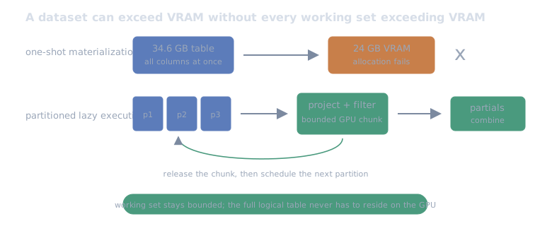
Logical dataset size and peak working-set size are different constraints. A partitioned plan can keep the latter below VRAM without pretending the former fits.

Four labels, three execution systems

The comparison needs one naming caveat before the numbers.

• DuckDB ran on eight CPU threads and returned Arrow.
• Polars CPU ran the same lazy query with its streaming CPU engine.
• Polars GPU sent that lazy plan to the RAPIDS cuDF-backed GPU engine.
• native cuDF expressed the operation directly with the eager cuDF API.

Polars GPU and native cuDF are not two unrelated GPU implementations. They are two ways of driving RAPIDS: one through an optimized lazy query plan and a partitioned streaming executor, the other through direct dataframe operations. The difference mattered most when the dataset grew beyond VRAM.

I disabled Polars’ transparent CPU fallback. An unsupported GPU query had to fail, not quietly produce a fast “GPU” result on the CPU. The timed region started before Parquet input and stopped only after a CPU-backed Arrow result was materialized. Every accepted result matched a canonical reference.

The box was the same RTX PRO 4000 Blackwell SFF with 24 GB VRAM. The pinned container used Python 3.12.13, DuckDB 1.5.5, Polars 1.42.1, cuDF 26.08.00, and PyArrow 23.0.1. Inputs were deterministic synthetic Parquet on local NVMe, warmed into the OS cache. Each condition had a warmup and three measured trials in seeded randomized order.

The public, output-complete notebook and its 196-row derived evidence table are in ramwise-examples. The notebook contains the charts and outputs; it does not need a GPU to read or rerun the analysis.

At 100,000 rows, Polars CPU won all seven workloads

At 100,000 rows, Polars CPU won all seven workloads. That is not surprising once the timed boundary is honest. The GPU has to initialize work, allocate, schedule kernels, and return a CPU-backed result. At this scale the useful query is over before there is enough parallel work to absorb the startup cost.

The first crossover arrived at five million rows, but only for the join:

Workload	First measured GPU win
join then group-by	5 million rows
12-column feature aggregation	10 million rows
projected scan and group-by	20 million rows
2-column feature aggregation	20 million rows
6-column feature aggregation	20 million rows
filtered top-k sort	no GPU win through 50 million
string filter and normalization	no GPU win through 50 million

That spread is the decision rule. Row count describes how much data exists; the plan describes how much parallel work survives projection, filtering, and the shape of the operator.

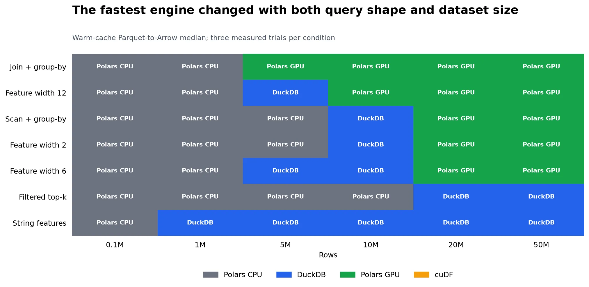
There is no vertical break-even line. Each query changes color at a different size, and two never reach the GPU in the measured range.

At fifty million rows, Polars GPU won the join, scan, and all three feature widths. DuckDB still won the string query and top-k sort.

50-million-row workload	Winner	Median	Lead over next engine
join then group-by	Polars GPU	0.108 s	1.55×
projected scan and group-by	Polars GPU	0.100 s	1.31×
12-column feature aggregation	Polars GPU	0.415 s	1.42×
filtered top-k sort	DuckDB	0.131 s	1.18×
string filter and normalization	DuckDB	0.089 s	1.09×

Even at the largest in-VRAM scale, two plausible analytical tasks preferred a compact CPU query engine. A routing rule based only on dataframe size would have sent both to the wrong place.

Unused width disappeared at projection

My first wide-table design was wrong in a useful way. I added columns, then ran a query that did not need them. Every competent engine projected them away. The table was physically wide and computationally narrow.

So the final width workloads calculate a feature score from two, six, or twelve metric columns before aggregation. Now width represents bytes decoded and arithmetic performed, not decorative columns in a schema.

At fifty million rows, Polars GPU took 0.158 seconds for two metrics, 0.261 for six, and 0.415 for twelve. It won all three. But its first win moved with the width: ten million rows for twelve columns, twenty million for two and six.

The wider query crossed earlier because it supplied more useful parallel work per row. That sounds obvious after the fact. It is also exactly what a single “GPU break-even row count” erases.

Snappy and Zstandard changed the winner

I also repeated three workloads at twenty million rows with Snappy and Zstandard. The codec changed the result, but not in a way that supports a universal ranking.

With Snappy, DuckDB won the twelve-column feature workload, Polars GPU won the scan, and Polars CPU won the string query. With Zstandard, Polars CPU won the feature and string workloads while DuckDB won the scan.

Codec cost was consumed inside the query plan. Compressed size, decoder implementation, projected columns, and the work after decoding interacted, so an isolated decompression leaderboard would not have predicted these winners.

Polars GPU finished the 34.6 GB workload

The last dataset had 200 million rows: 19.7 GB of Parquet and 34.6 GB of estimated logical data, about 1.34 times the GPU’s nominal capacity.

Native cudf.read_parquet over the complete file set failed. Even with generic cuDF spilling enabled, it requested one 23.3 GB device allocation and ran out of VRAM. The setting was real; the guarantee I had mentally attached to it was not. RAPIDS documents spilling as a buffer-management mechanism and describes the device threshold as a soft limit. It cannot make every monolithic allocation divisible.

I kept that failure in the public evidence and added a deliberately named cudf-streaming control: read one file at a time, calculate exact partial sums and counts on the GPU, then merge the tiny aggregates. It completed, but took 13.93 seconds.

The normal Polars GPU query completed in 1.54 seconds. Polars CPU took 1.85 seconds and DuckDB 2.28.

200-million-row path	Median	Relative time
Polars GPU streaming	1.538 s	1.00×
Polars CPU streaming	1.854 s	1.21×
DuckDB	2.278 s	1.48×
manual native-cuDF partitions	13.931 s	9.06×
native cuDF one-shot read	failed	CUDA out of memory

That is not a contradiction inside RAPIDS. The cuDF-backed Polars engine had a partitioned query graph; the eager native-cuDF call tried to materialize the input. My manual loop had bounded memory but paid Python/API overhead eighty times and surrendered cross-partition planning.

Both GPU paths ultimately used cuDF, yet their execution models produced a ninefold difference and one of them ran out of memory.

A routing policy for this box

I would not build a router that says “above ten million rows, use the GPU.” The experiment rejects that rule.

I would use something closer to this:

1. Project and filter before choosing an engine. Work removed by the query optimizer beats accelerated work.
2. Keep DuckDB or Polars CPU for small, selective, string-heavy, and top-k paths. They won meaningful parts of this matrix, not merely toy cases.
3. Use Polars GPU when a supported lazy plan has enough surviving work—joins, scans, and wide feature preparation here—and make fallback fail loudly while validating the route.
4. For data near or beyond VRAM, choose a documented streaming or distributed execution plan. A spill flag is memory policy, not proof that an eager algorithm is out-of-core.
5. Keep results on the GPU when the next stage belongs there. This benchmark paid to return a CPU-backed Arrow result, so it is conservative for a GPU-resident continuation and realistic for a CPU consumer.
6. Benchmark the full query at representative sizes. Engine, codec, width, selectivity, storage, and output placement can all move the boundary.

There are still limits. This was warm-cache local NVMe, synthetic data, fixed versions, one workstation, and three measured trials per condition. It did not test remote object storage, cold cache, thousands of tiny files, energy use, or multi-GPU execution. The Polars GPU engine is also still documented as open beta, so its supported plan surface and performance will move.

These measurements support a practical split. After projection and filtering, supported joins, scans, and wide feature calculations can justify Polars GPU. Small queries, strings, and top-k work can remain with Polars CPU or DuckDB. Datasets near VRAM capacity need an execution plan that partitions the work; enabling spill on an eager materialization is not equivalent.

Sources and reproducibility

• Output-complete notebook and sanitized evidence
• Polars GPU support and strict raise_on_fail behavior
• cuDF-Polars streaming execution model
• cuDF spilling behavior and soft device limits
• DuckDB Parquet projection and filter pushdown

More on Data engineering How Much of a Spark Plan Actually Runs on the GPU? →