100 Million Points on One GPU
A point-in-polygon benchmark can make the GPU look inevitable.
Put millions of points beside a handful of polygons, run the same geometry test many times in parallel, and report the largest speedup. The result may be true. It can still hide the decision that matters.
Spatial systems rarely test every pair. They filter with bounding boxes or a tree, refine the surviving candidates with an exact predicate, and then return the matches. The index changes how much work reaches the geometry kernel. It also adds construction, memory, and data-placement costs of its own.
The benchmark therefore covered the whole plan.
Those plans sit underneath geofencing GPS pings, matching trips to service areas, measuring insurance or disaster exposure, analysing mobility, and finding the nearest road or asset. Some are repeated against a stable polygon index; others build an index for one batch. Point count alone cannot tell an operator whether the GPU will repay that surrounding work.
On an RTX PRO 4000 Blackwell SFF, cuSpatial’s indexed point/polygon join was 5.27× slower than an eight-thread Shapely/STRtree plan at 100,000 points. At one million points it was 2.09× faster. At one hundred million it was 15.40× faster.
But a simple rectangular window did not cross until one hundred million points, where the GPU led NumPy by only 1.04×. And nearest-feature search was usually a CPU win in the fully verified 100,000-point range unless the lines became complex.
The indexed workload justified the GPU once enough exact geometry survived the filter to repay data placement and tree construction. The rectangular window needed two orders of magnitude more points, and the nearest-feature path hit a correctness limit before it produced a larger-scale performance claim.
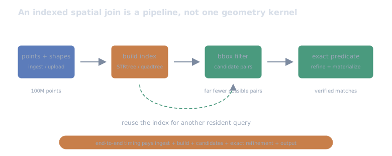
The fast geometry predicate sits near the end. A one-shot decision also pays for ingest and index construction; a resident repeated query can reuse both.
Four plans, not one spatial benchmark
The deterministic data lived in the unit square. I varied point count, polygon count, vertices per polygon, polygon radius, line count, and vertices per line. The four operations were:
- a rectangular point window;
- direct point-in-polygon against 16 polygons;
- indexed point/polygon join; and
- indexed nearest-linestring search.
The CPU alternatives were NumPy for the window and Shapely 2.0.7 with GEOS 3.13.1 for geometry. Indexed and nearest CPU queries used eight fixed threads; Shapely generally releases the GIL around GEOS work and documents STRtree’s bounding-box-first behavior. The GPU used cuSpatial and cuDF 25.04 in NVIDIA’s digest-pinned RAPIDS CUDA 12.8 image.
That version needs an explicit warning. NVIDIA currently lists cuSpatial under its inactive RAPIDS projects, with 25.04 as the final stable documentation. This is an evaluation of that fixed historical release, not a recommendation to build a new platform around an actively advancing library.
Each published case has three randomized fresh-process replications. Each process ran one warmup and three measured trials. GPU regions synchronized at both boundaries. I timed ingest, index construction, candidate generation, exact refinement, and result materialization separately.
The public companion in
ramwise-examples
contains the output-complete notebook, 33-row confirmed table, three explicit
exclusions, targeted correctness controls, full harness, digest-pinned image,
and exact Conda package specification.
Indexed point-in-polygon crossed between 100K and 1M
With 1,024 polygons of 17 vertices each, the end-to-end indexed result was:
| Points | CPU STRtree | GPU quadtree | GPU speedup |
|---|---|---|---|
| 100K | 19.56 ms | 103.14 ms | 0.19× |
| 1M | 194.21 ms | 92.97 ms | 2.09× |
| 10M | 1.851 s | 0.214 s | 8.67× |
| 50M | 8.941 s | 0.659 s | 13.56× |
| 100M | 18.412 s | 1.196 s | 15.40× |
I did not test enough values to claim an exact crossover point. It lies somewhere between the measured 100K and 1M cases for this geometry, hardware, and software stack.
The direct, unindexed point-in-polygon path crossed sooner. It was already 1.42× faster at 100K and reached 11.39× at 10M. That is not a contradiction. The direct case had only 16 polygons and no quadtree to build. At small scale, adding the “better” indexed GPU plan cost more than the work it removed.
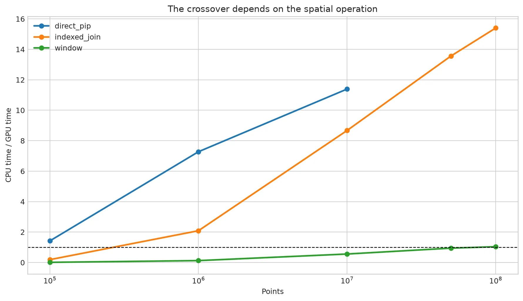
The dashed line is parity. Each point is the median of three fresh-process replications; the public CSV also includes each replication range.
A resident query crossed before the lifecycle did
At 100K indexed points, the GPU query itself took 5.34 ms against 6.57 ms on the CPU: a modest 1.23× resident win. The end-to-end GPU path still took 103.14 ms because ingestion and quadtree construction dominated the first query.
If both sides kept their data and indexes resident, the GPU needed about 68 queries to repay its larger fixed-cost difference.
At one million points the first full lifecycle already favored the GPU. The CPU had to materialize one million Shapely point geometries; the GPU’s upload and quadtree cost was no longer the larger bill.
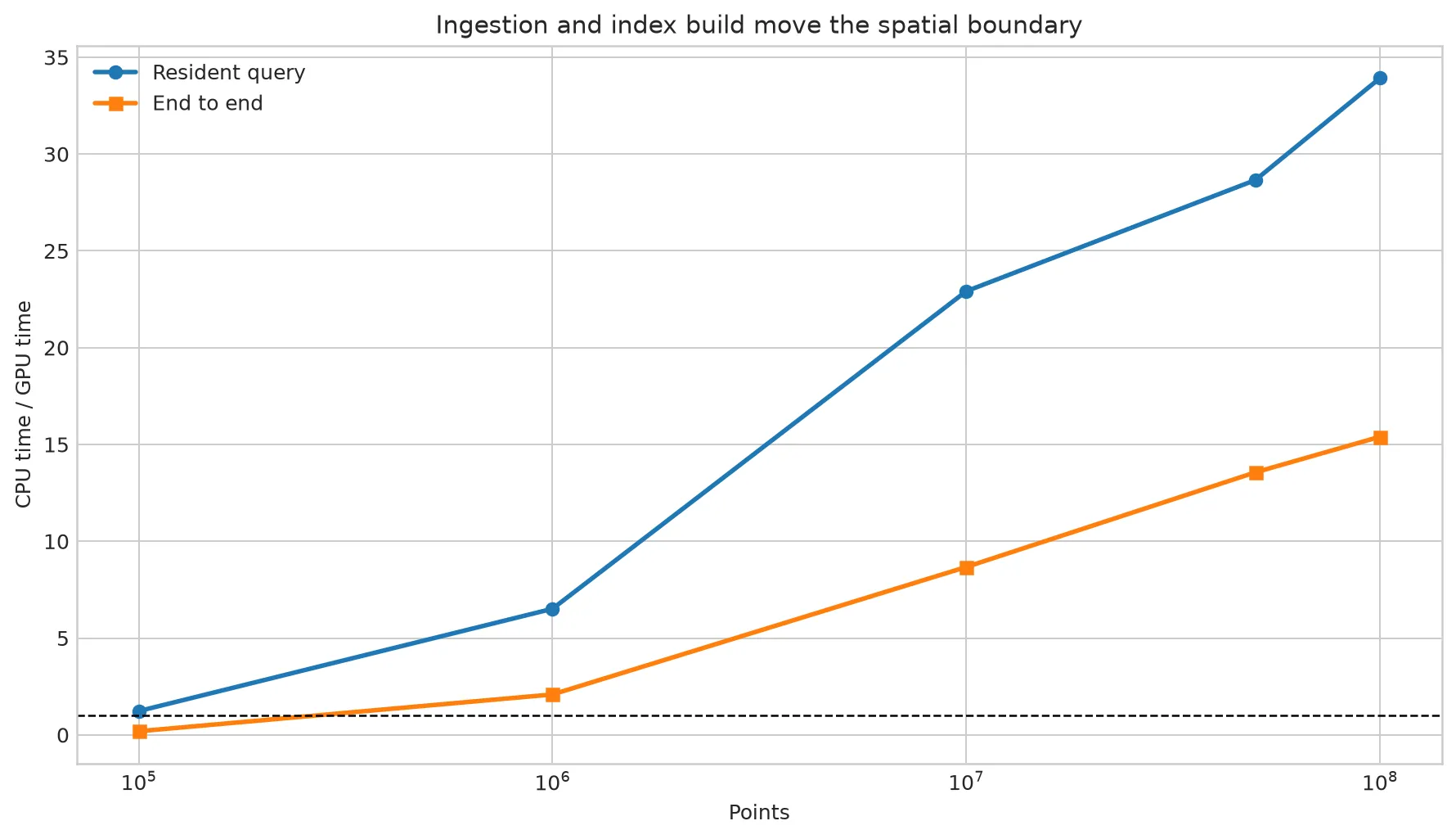
Build time cannot simply be added or omitted by convention. Its place in the timer depends on the workload lifecycle:
one-shot = ingest + index build + query + materializationreused = fixed costs once + N × repeated query costFor an interactive map that reuses a stable resident index, repeated-query economics matter. For a batch that loads coordinates, joins once, and exits, the one-shot boundary is the honest one.
More polygon vertices reduced the GPU lead
At 10M points, increasing each polygon from 4 to 257 vertices reduced the indexed GPU speedup from 8.90× to 5.61×.
| Vertices per polygon | CPU | GPU | GPU speedup |
|---|---|---|---|
| 4 | 1.808 s | 0.203 s | 8.90× |
| 17 | 1.848 s | 0.216 s | 8.55× |
| 65 | 1.953 s | 0.247 s | 7.90× |
| 257 | 2.172 s | 0.387 s | 5.61× |
Both plans first found bounding-box candidates, then ran exact geometry on the survivors. cuSpatial describes the same trade explicitly: quadtree pre-filtering can dramatically reduce point tests, at the cost of the tree, sorted point indices, and extra memory. Shapely’s STRtree similarly returns bounding-box intersections and optionally refines them with a predicate.
The GPU still won every confirmed 10M indexed-join condition. But its exact stage grew faster as the polygons became more detailed. More vertices did not simply create “more parallel work”; they changed the balance between candidate filtering and exact refinement.
Polygon count had a different effect. From 16 to 4,096 polygons, the match count stayed around 4.44M, but GPU candidates rose from 6.30M to almost 10.0M. The speedup fell from 9.31× to 6.41×. The index was still helpful, but its false-positive work changed with the geometry layout.
NumPy nearly matched cuSpatial at 100 million points
The rectangular window was deliberately cheap: four NumPy comparisons and a Boolean mask versus cuSpatial’s window operation plus transfer and result handling.
| Points | NumPy | cuSpatial | GPU speedup |
|---|---|---|---|
| 100K | 0.513 ms | 39.505 ms | 0.013× |
| 1M | 5.768 ms | 45.463 ms | 0.13× |
| 10M | 69.726 ms | 124.625 ms | 0.56× |
| 50M | 365.957 ms | 387.235 ms | 0.95× |
| 100M | 730.088 ms | 702.179 ms | 1.04× |
Even at 100M points, the end-to-end win was within four percent. The resident GPU query was 1.43× faster there, but needed about ten repeated queries to recover the one-time placement difference.
Point count alone did not supply enough work. The GPU needed enough arithmetic or repeated queries per transferred byte. A vectorized CPU predicate therefore remained competitive at a scale where the more expensive geometry predicate already favored the GPU by an order of magnitude.
A 129-vertex line moved nearest search to the GPU
I bounded nearest-linestring performance claims to the range that passed pointwise correctness. At 100K points, changing the number of nine-vertex lines from 16 to 1,024 left the GPU slower end to end: 0.51× to 0.81× the CPU result depending on the case.
Changing line complexity moved the boundary more sharply:
| Vertices per line | CPU | GPU | GPU speedup |
|---|---|---|---|
| 2 | 38.66 ms | 79.61 ms | 0.49× |
| 9 | 40.33 ms | 78.60 ms | 0.51× |
| 33 | 68.46 ms | 80.33 ms | 0.85× |
| 129 | 198.58 ms | 87.04 ms | 2.28× |
The GPU’s fixed costs stayed visible, while the CPU distance work grew with the number of segments. The crossover came from geometry complexity rather than a larger point set.
I did not extend that speedup curve to one million points because the numerical
control failed there. At 100K, four candidate-box radii produced complete
results with zero mismatches at rtol=atol=1e-10; maximum absolute error was
3.46e-11. At 1M, the same 11 rows differed by as much as 9.25e-4 at every
tested radius. Widening the candidate envelope did not fix it.
I excluded the larger nearest-feature cases rather than turn that numerical disagreement into a performance claim.
One quadtree setting silently dropped 94,712 points
The most important catch appeared before the confirmation matrix.
At 10M points, quadtree leaf capacity 128 returned a permutation with only 9,905,288 points represented in leaf lengths. The indexed join produced 245 matches instead of the CPU reference’s 4,444,679. Increasing the capacity to 256 accounted for all 10M points and reproduced every pair signature.
The harness therefore refuses to time an indexed GPU case unless both the point permutation and the sum of leaf lengths equal the input point count. Published joins also require CPU/GPU match counts and two independent order-independent 64-bit pair reductions to agree in all three replications.
Two CPU stress replications exposed a separate stability boundary. Shapely/ GEOS exited with code -11 for one 10M × 16,384-polygon replication and one very-high-overlap replication. The other two processes finished, but the entire cases are excluded from performance claims. Partial success is not a median.
Operational choices from this benchmark
For workloads shaped like these, I would use five rules:
- Keep NumPy on the CPU for one-shot rectangular filtering unless scale is enormous or the data already lives on the GPU. At 50M points, the full GPU lifecycle still lost.
- Use direct GPU point-in-polygon for a small fixed polygon set. Avoid paying for an index whose construction removes too little work.
- Use an indexed GPU join for million-scale and larger point sets when exact refinement is substantial. On this box, the confirmed boundary moved from a 5.27× loss at 100K to a 2.09× win at 1M.
- Measure resident reuse separately from one-shot execution. A GPU query can win while its first lifecycle loses; at 100K, the measured repayment was about 68 queries.
- Make index coverage and pointwise geometry checks release gates. An incorrect spatial result is not an acceleration, and a failed replication cannot support a speedup claim.
The scope here is narrow: deterministic synthetic 2D Cartesian geometry already in host memory, one workstation GPU, fixed CPU affinity, and a retired cuSpatial release. It did not include file parsing, GeoParquet, coordinate transforms, invalid real-world polygons, spherical distance, spatial skew, index updates, multi-GPU execution, or a contemporary supported GPU GIS stack.
The vector-search note, How Many Queries Pay for a Vector Index?, applies the same build-versus-query accounting to a different index.
Because cuSpatial is now inactive, I would carry forward the experimental method more readily than this exact library choice: separate lifecycle stages, count candidates, calculate index reuse, and reject timings when geometry does not match. A current production evaluation would need to repeat those controls against a supported GPU GIS stack.
Move the polygon; watch the exact matches
Drag a polygon through a clustered point field while the exact point-in-polygon predicate runs on WebGPU.