I built a GPU data-engineering box and started with a straightforward question: could it read Parquet faster than a CPU?

That question comes up whenever an ETL job scans lakehouse partitions, a notebook projects a few fields from a wide table, or a feature pipeline loads training data. In each case, the useful choice is not simply “use the faster reader.” Startup cost, decompression, column projection, and where the data needs to go next can change the answer.

At fifty million rows, it did. cuDF beat PyArrow, pandas, Polars, and DuckDB in every full-sized condition I tested. Under isolated CPU cores, its median lead over the fastest CPU reader was 2.16×, with individual conditions ranging from 1.19× to 3.10×.

The smaller run had already complicated that answer: PyArrow kept two projected cases at five million rows. More importantly, the largest improvement anywhere in the study came from asking for fewer columns, not from changing engines or codecs. The row-group layout that gave cuDF its fastest result also penalized a projected PyArrow read.

For this box, cuDF earned its place on large scans. The amount of work handed to it—and whether the next stage stayed on the GPU—determined how valuable that choice was.

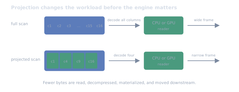
Projection changes the amount of data that must be read, decompressed, materialized, and moved before CPU-versus-GPU speed becomes the question.

How I tried to make the comparison fail

The first version was deliberately small: five readers—PyArrow, pandas, Polars, DuckDB, and cuDF—over deterministic synthetic Parquet. I varied three schema shapes:

• a narrow numeric table;
• a mixed table with strings and nulls; and
• a wide table with sixteen additional floating-point metrics.

Each shape was written uncompressed, with Snappy, and with Zstandard. Each was read both in full and with a four-column projection. Timed reads included decode and materialization into the engine’s returned frame. GPU work was synchronized before stopping its timer. Every result was checked against a full-column aggregate signature outside the timed region.

I also did the parts benchmark screenshots tend to omit:

• warmups before measured trials;
• seeded random trial order;
• independent process-level replications;
• continuous 20 ms GPU telemetry;
• later, host CPU telemetry and explicit CPU affinity; and
• immutable raw JSON with a resumable case state.

The test box ran Ubuntu 26.04 with an NVIDIA RTX PRO 4000 Blackwell SFF (24 GB), driver 595.71.05, CUDA 13.1, RAPIDS 26.08, and Python 3.12. CPU-isolated runs used eight Core Ultra 9 285HX performance cores. Files lived on the machine’s NVMe data volume and were warmed into the OS cache before measurement.

The public reproduction bundle lives in ramwise-examples. Its notebook/ child contains the approachable teaching example; full-benchmark/ contains the sanitized complete harness, study configs, locked environment, methodology, tests, and derived results. Ubuntu 26.04 was the host; the benchmark ran inside a digest-pinned Ubuntu 24.04 CUDA container. Raw host telemetry and private infrastructure details are intentionally not published.

The five-million-row smoke exposed the startup cost

The 5-million-row compatibility smoke was not supposed to make performance claims. It was there to catch broken combinations before a longer run. It caught something more useful: PyArrow beat cuDF in two narrow projected conditions.

For uncompressed numeric data, PyArrow finished in 13.9 ms and cuDF in 15.1 ms. For numeric Zstandard, PyArrow took 18.6 ms and cuDF 22.4 ms. Those are small differences at small runtimes, so I treated them as evidence of a startup floor rather than a declaration that either reader was categorically faster.

A GPU read has fixed work to amortize: dispatch, allocation, library setup, and synchronization. If the useful read is only a few columns and a few milliseconds, the parallel machine may run out of work before it runs out of overhead.

Accordingly, the claim here is limited to the fifty-million-row workloads I measured. Locating the crossover between the two tested scales requires a separate size sweep.

At fifty million rows, cuDF won all eighteen conditions

The full exploratory matrix ran 3 profiles × 3 codecs × 2 projections × 3 replications: fifty-four cases, each with a warmup and five measured trials per engine. PyArrow was the fastest CPU reader in every condition. cuDF was faster than it in all eighteen profile/codec/projection combinations.

Its median advantage was 1.78×, ranging from 1.36× to 2.77×. The companion repository includes the complete sanitized 90-row table behind those claims: all five engines across all eighteen conditions.

Then I made the CPU comparison stricter. The host is an Intel Core Ultra 9 285HX: logical CPUs 0–7 are its eight 5.5 GHz performance cores, while 8–23 are efficiency cores. I pinned the benchmark container to 0–7, kept every engine at eight requested threads, and sampled the process, the selected cores, and the whole host alongside the GPU.

The targeted confirmation repeated mixed and wide data, Snappy and Zstandard, full and projected reads, with three replications each. Background activity on the selected cores stayed low: a median of 0.22 core and a maximum of 0.34 core across the report rows.

Shape	Codec	Read	cuDF	PyArrow	cuDF lead
mixed	Snappy	all	0.126 s	0.392 s	3.10×
mixed	Snappy	projected	0.093 s	0.220 s	2.35×
mixed	Zstandard	all	0.128 s	0.347 s	2.70×
mixed	Zstandard	projected	0.115 s	0.226 s	1.96×
wide	Snappy	all	0.588 s	0.699 s	1.19×
wide	Snappy	projected	0.093 s	0.222 s	2.38×
wide	Zstandard	all	0.833 s	1.482 s	1.78×
wide	Zstandard	projected	0.115 s	0.228 s	1.98×

Isolation did not make the GPU result disappear. The median lead in this targeted set was 2.16×. More importantly, it removed the easiest objection: the CPU readers were not being compared while accidentally wandering across a hybrid core topology or competing with an invisible workload.

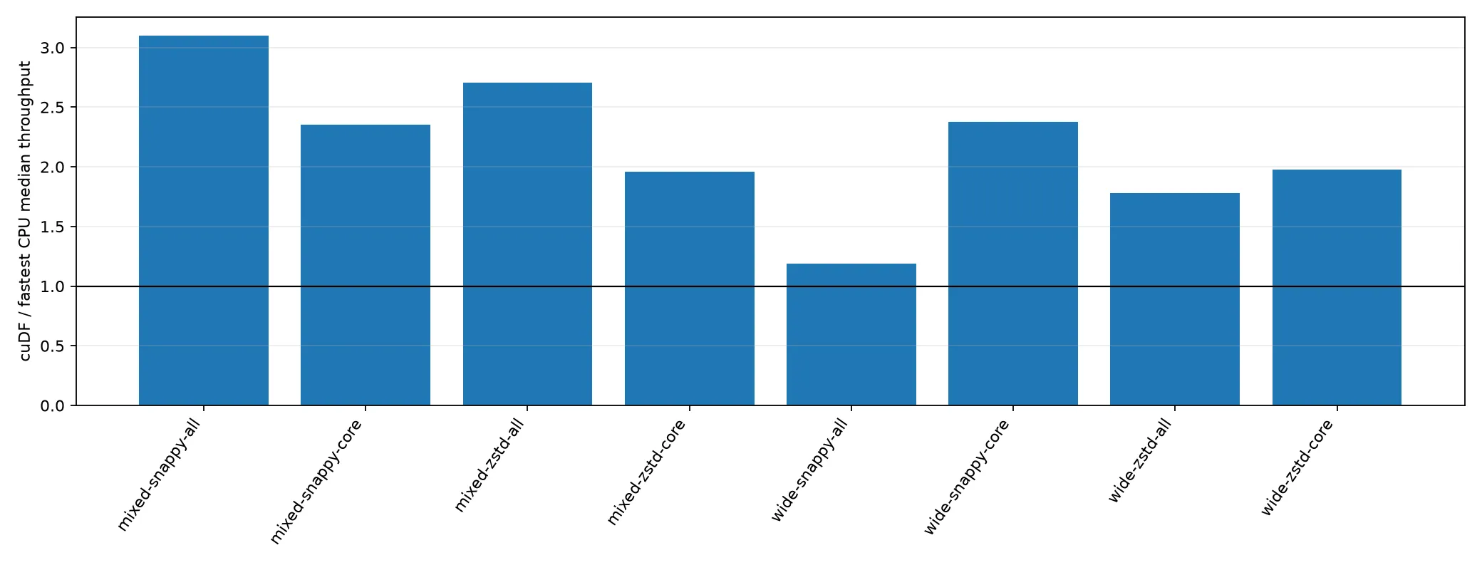
Every isolated 50-million-row condition stayed above the 1× break-even line.

Reading four columns cut cuDF time by 6–7×

On the narrow numeric table, projection barely helped cuDF. There were not many columns to avoid. On the wide table, reading four columns instead of all twenty-two reduced cuDF elapsed time by roughly 6× to 7×.

That gain was several times larger than the typical GPU-over-CPU difference.

This is the part that changes an application design. If a query needs four columns, the first optimization is not “buy a GPU” or “change the codec.” It is to make sure the reader asks for four columns. A fast engine reading unwanted data is still doing unwanted work.

There is an important measurement trap here. The benchmark reports compressed file MiB divided by elapsed time. For a projected read, that is a useful comparative rate, but it is not physical disk bandwidth: the numerator includes columns the reader did not materialize. I use elapsed seconds for the projected interpretation.

A 262,144-row group balanced CPU and GPU reads

The final experiment fixed the hardest wide/Zstandard case at fifty million rows and varied only the row-group size: 65,536; 262,144; 1,048,576; and 2,500,000 rows. The files had 2.5 million rows each, so the last option was one row group per file.

The compressed file size barely moved—less than 0.05%. This was reader overhead, not a compression story.

Rows per group	cuDF all	PyArrow all	cuDF projected	PyArrow projected
65,536	0.826 s	1.689 s	0.158 s	0.331 s
262,144	0.819 s	1.476 s	0.116 s	0.228 s
1,048,576	0.819 s	1.485 s	0.120 s	0.230 s
2,500,000	0.775 s	1.481 s	0.114 s	0.348 s

Small groups lost. Compared with 262,144 rows, the 65,536 layout made full PyArrow 14% slower, projected PyArrow 45% slower, and projected cuDF 36% slower.

One group per file gave cuDF its best observed numbers: about 5% faster on full reads and 2% faster on projection than the 262,144 baseline. But that same layout made projected PyArrow 52% slower.

So there are two answers:

• 262,144 rows per group is the balanced default for data shared by CPU and GPU readers.
• One group per file is a plausible cuDF-only full-scan optimization, worth considering when that access pattern is known and stable.

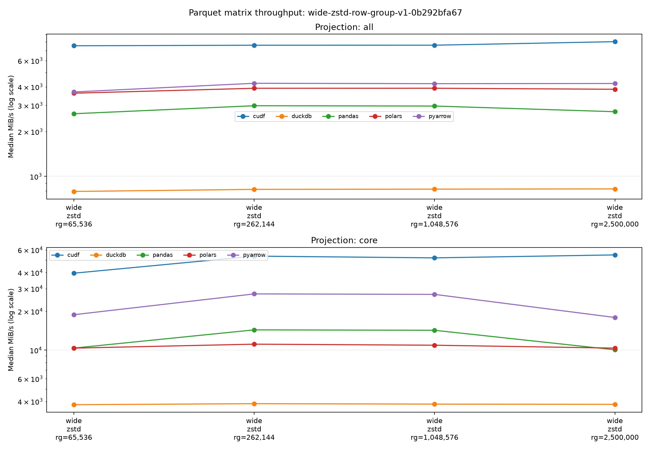
The smallest groups add overhead. The largest groups favor cuDF but penalize projected PyArrow, leaving 262,144 as the balanced result for this dataset.

The tiny 2% projected cuDF difference is not something I would build policy around. There were only three independent replications. The 262,144 projected condition varied by under 1% for both PyArrow and cuDF, while the smallest-group cuDF projection varied much more. “Near-optimal and stable across engines” is a better default than “won one median by two milliseconds.”

A practical policy for this workload

On this hardware I would first remove unnecessary I/O, then choose the engine that fits the remaining work and its downstream destination. Five practical rules follow from the measurements.

1. Reduce the work before accelerating it. Push column projection and predicates into the Parquet reader. Projection produced the largest improvement here because work that is never read does not have to be decompressed, decoded, allocated, or transferred. Both PyArrow and cudf.read_parquet support projection and predicate pushdown; Parquet row-group statistics can eliminate irrelevant groups before their data is materialized.

2. Choose an execution path for the pipeline, not for one operator. cuDF is most compelling when the input is large enough to expose GPU parallelism and the following filters, joins, aggregations, feature engineering, or model training also run there. If the result must immediately return to CPU memory, some of the read-time win can disappear into conversion and transfer overhead. RAPIDS accordingly emphasizes end-to-end GPU workflows rather than isolated accelerated calls.

3. Treat small reads as a CPU workload until measurements say otherwise. A GPU has an entrance fee: initialization, allocation, kernel launch, decoder setup, and data movement. PyArrow can therefore remain faster for small files, narrow projections, selective queries, and interactive reads even when cuDF wins decisively on large scans. A GPU needs enough useful work, not merely a Parquet file.

4. Size row groups by bytes and access pattern—not by a universal row count. Small groups improve pruning granularity and scheduling flexibility, but too many add metadata, dispatch, and decoder overhead. Large groups favor sequential scans and give the GPU more work per launch, but can waste reads when predicates are selective and can increase peak-memory pressure. Apache Parquet’s configuration guidance likewise describes row-group sizing in bytes and explicitly frames large groups as a sequential-I/O optimization. A broad VLDB evaluation of Parquet and ORC also found that encoding, metadata, filtering, and hardware all affect scan behavior.

   On this dataset, 262,144 rows was the best shared CPU/GPU compromise. That is a useful starting point for similarly shaped data, not a format-wide prescription. Because row width and compression vary, another dataset’s 262,144 rows may represent a completely different number of bytes. One group per file remains a specialized option for stable cuDF-only full scans—not a general default.

5. Keep a strong CPU path. PyArrow is not merely an emergency fallback. It is the natural execution path for small or selective reads, CPU-resident downstream work, machines without a compatible GPU, and correctness comparisons. A practical system can choose between CPU and GPU instead of forcing every read through one engine.

The experiment does not establish a universal break-even row count. Warm cache, local storage, file count, schema width, codec, projection, selectivity, GPU generation, VRAM pressure, and downstream placement can all move that boundary. Cold object storage or thousands of tiny files may make storage and metadata latency dominant; data larger than VRAM may require chunked or distributed execution.

The missing size sweep prevents a single numeric threshold, but it does not prevent a working policy for this machine. PyArrow remains the sensible path for small, selective, or CPU-bound reads. cuDF is attractive for sufficiently large scans when later work can remain on the GPU. Projection, pruning, and file layout should be settled before either engine is asked to do the work.

More on Data engineering How Much of a Spark Plan Actually Runs on the GPU? →