DuckLake on One Machine
I wanted to see how much of a normal data-engineering project could fit around DuckLake on one machine.
The stack was small: DuckDB ran the SQL, DuckLake supplied the catalog, Parquet storage, and snapshots, and marimo supplied Python notebooks. I used a thin filesystem-backed runner for projects, scheduled jobs, and retained notebook output. That runner is my own project, currently called Anatini. It is the plumbing around this experiment, not something the reader needs to know beforehand.
I made one job that behaved like a small data platform. It generated source files, loaded them, cleaned and modeled orders, applied inserts and updates and deletes, processed nested JSON events, quarantined bad rows, ran quality checks, and queried an older snapshot. Then I ran the same job at four sizes.
The smallest version had 100,000 orders and 200,000 events. The largest had 50 million orders and 100 million events.
On my desktop, the large version finished in a median 4 minutes 48 seconds. Peak sampled process memory was 3.33 GiB. All 20 measured runs passed all 16 checks.
The engine held up better than I expected. Two other numbers bothered me more. A quick run did about five seconds of data work but took about a minute to finish because the runner retained nine notebook outputs. And after 24 runs, 7.11 GiB of current DuckLake data had left 61.32 GiB in the lake directory because I had not expired any old snapshots.
I would rather find those problems now than after putting the job on a schedule.
The job
The main marimo notebook called eight child notebooks through the same path used by a scheduled job.
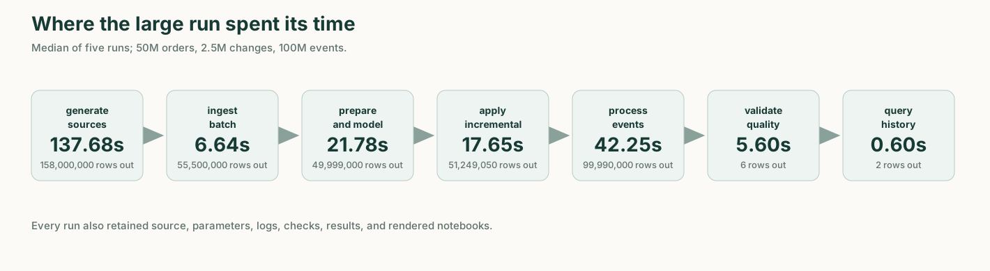
Median step times from the large profile. An eighth child notebook saved the measurements and chart.
The generator wrote five deterministic sources: orders and customers as Parquet, products and order changes as CSV, and nested events as JSONL. The rest of the job did the following:
- loaded the batch into DuckLake;
- typed and standardized the orders;
- split deliberately bad records into quarantine tables;
- built an order fact and daily sales aggregate;
- applied overlapping inserts, updates, deletes, and late changes;
- parsed and sessionized the event stream;
- reconciled counts, dimensions, quarantine rows, and revenue; and
- compared the order state before and after the changes.
I chose this shape because scan benchmarks skip most of it. The job included different file formats, writes, replacements, keyed changes, joins, bad data, history, and enough retained output to debug an old run.
The responsibilities stayed plain. DuckLake kept its catalog in SQLite and its table data in Parquet. marimo notebooks remained Python files. The runner stored job definitions and historical output as project files rather than hiding the experiment in another service.
How I ran it
I used four profiles:
| Profile | Base orders | Changes | Events | Customers | Products |
|---|---|---|---|---|---|
| quick | 100,000 | 5,000 | 200,000 | 10,000 | 1,000 |
| small | 1,000,000 | 50,000 | 2,000,000 | 100,000 | 10,000 |
| medium | 10,000,000 | 500,000 | 20,000,000 | 1,000,000 | 100,000 |
| large | 50,000,000 | 2,500,000 | 100,000,000 | 5,000,000 | 500,000 |
I did one exploratory quick run, locked the workload and protocol, then gave each profile one warm-up and five measured runs. Large was conditional on medium fitting inside the time, memory, and disk limits I set beforehand. It did, so large ran without changing the SQL or data shape.
Runs were serial. DuckDB had four threads and a 6 GB memory limit. I did not flush the Windows page cache, so these are normal warm-workstation numbers, not cold-storage numbers. Each notebook timed the work it owned with time.perf_counter_ns(). The runner’s timestamps measured the complete job, including launching child notebooks and retaining their output.
The machine was a Ryzen 9 5950X with 128 GiB RAM and a Sabrent Rocket 4.0 NVMe SSD, running native Windows 11. The measured versions were DuckDB 1.5.5, DuckLake extension d8a1881e, marimo 0.23.16, CPython 3.14.6, and the Anatini 0.9.0 runner. Docker and WSL were not involved.
This is a generous desktop. I am recording what happened on it, not predicting what the same job will do on a 16 GB laptop.
What happened
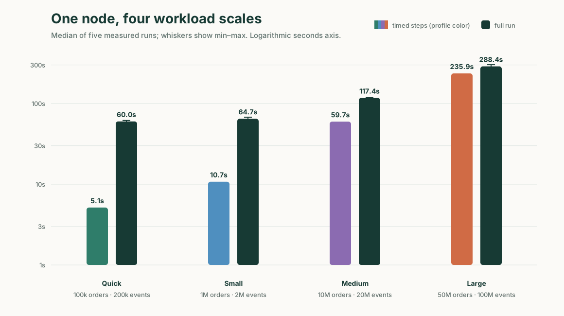
Five measured runs per profile. Whiskers show the minimum and maximum. The time axis is logarithmic.
| Profile | Data work | Complete run | Run range | Peak RSS | Current data |
|---|---|---|---|---|---|
| quick | 5.141 s | 59.985 s | 58.395–61.654 s | 0.215 GiB | 0.012 GiB |
| small | 10.748 s | 64.718 s | 57.150–67.716 s | 0.313 GiB | 0.137 GiB |
| medium | 59.653 s | 117.377 s | 117.087–119.680 s | 0.815 GiB | 1.422 GiB |
| large | 235.878 s | 288.435 s | 252.569–302.288 s | 3.329 GiB | 7.111 GiB |
Medium was remarkably steady: all five complete runs landed between 117.087 and 119.680 seconds. Large moved around more, from 4 minutes 13 seconds to 5 minutes 2 seconds.
The final large state contained 51,249,050 accepted current orders, 99,990,000 accepted events, 10,000 quarantined events, and 14,285,715 sessions. The older snapshot contained 49,999,000 accepted orders. The count and revenue reconciliations passed every time.
The history notebook compared aggregate state across the old and current snapshots in a median 0.600 seconds. I only use that number as a correctness and usability check. One fixed aggregate says nothing broad about time-travel performance.
Keeping notebook history added about a minute
The gap between the notebook timers and the complete run was surprisingly flat:
| Profile | Extra time around the data work |
|---|---|
| quick | 54.629 s |
| small | 55.427 s |
| medium | 59.089 s |
| large | 50.222 s |
I did not instrument that minute deeply enough to divide it among process startup, marimo execution, orchestration, run persistence, and HTML rendering. It is probably a mixture, and the benchmark cannot say how much belongs to each part.
The time bought something real. Every run kept the root notebook and all eight children with their source, parameters, console output, displayed results, checks, provenance, and historical HTML. I can open an old run and inspect what each notebook showed at the time.
Still, adding 55 seconds to a five-second job is a poor bargain. Adding roughly the same amount to a four-minute job is less objectionable. The runner needs a lighter retention option for short jobs; that went onto my list after this test.
The event count hid the expensive part
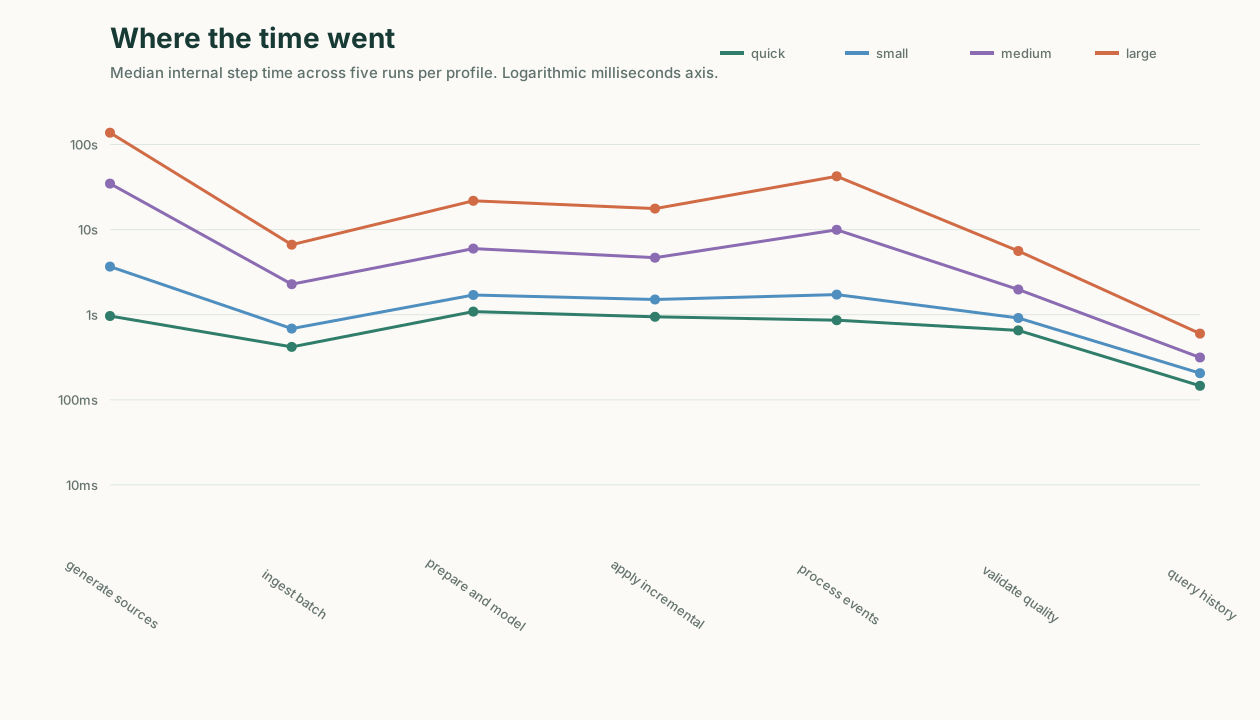
The vertical axis is logarithmic. File generation, JSON processing, modeling, and changes scale differently.
For the large profile, the median step times were:
| Step | Median |
|---|---|
| generate five source files | 137.676 s |
| process and sessionize events | 42.253 s |
| prepare, quarantine, and model | 21.781 s |
| apply 2.5M changes | 17.649 s |
| ingest facts and dimensions | 6.638 s |
| validate quality | 5.599 s |
| compare historical/current state | 0.600 s |
The 100-million-event step was not the slowest part. Generating all five source datasets took more than half of the timed work.
Batch ingestion accepted 55.5 million fact and dimension rows at about 8.36 million input rows per second. Event processing handled roughly 2.37 million rows per second. Preparation and modeling handled about 2.30 million. Applying the change file managed about 142,000 records per second while updating a 50-million-row current table.
I would not combine those rates into a single DuckLake score. A compressed Parquet load, JSON parsing, a dimensional join, table replacement, keyed changes, and quality aggregates are different jobs. The operation mattered more than the headline row count.
Old snapshots accumulated quickly
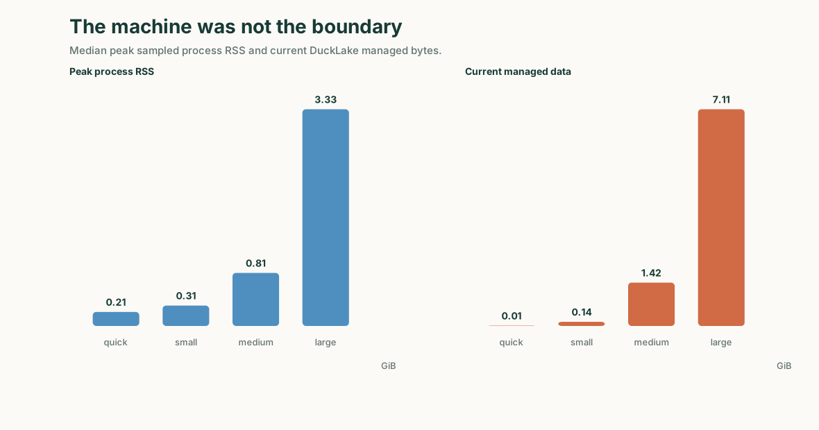
Median values from five runs. The large job stayed inside its four-thread, 6 GB DuckDB profile.
Memory was uneventful. Large sampled between 3.320 and 3.341 GiB peak RSS, well below both the DuckDB setting and the machine’s physical memory.
Disk was the part I would not leave unattended. The suite repeatedly replaced tables and applied changes, and I deliberately ran no snapshot expiry or compaction between repetitions. At the end:
- DuckLake was at snapshot 533;
- the lake contained 571 physical files;
- the project lake occupied 61.317 GiB; and
- files belonging to the current tables occupied 7.111 GiB.
That 8.6× difference is specific to this mutation-heavy run history. It is not a general DuckLake storage multiplier, and I did not capture a clean pre-suite disk baseline that would support one.
It does make the maintenance requirement hard to ignore. If I schedule this job, I also need to decide how long old snapshots remain reproducible, when their files expire, and how disk growth is reported. DuckLake already exposes current and snapshot-specific file membership, so cleanup should follow catalog metadata rather than whatever files happen to be visible in the directory.
Would I use it for real work?
For one developer and bounded local jobs, yes. The project was easy to inspect: notebooks were Python, SQL stayed SQL, tables were a SQLite catalog plus Parquet, and retained runs were ordinary artifact directories. I did not need Spark, Airflow, Kafka, an object store, or another database just to run this project.
I would stop treating this as enough when I needed multiple active writers, high availability, elastic concurrency, centralized governance, remote object storage, or several teams sharing ownership. None of those problems waits for the row count to become large, and this experiment did not test them.
I also have not tested cold-cache behavior, failure recovery in the middle of a commit, or the same profiles on ordinary 16–32 GiB machines. Those are separate experiments.
The practical result is fairly modest: on this workstation, this particular DuckLake-based data platform stayed correct and comfortable through 50 million orders and 100 million events. The next engineering work is in the surrounding platform: lighter run retention and deliberate snapshot housekeeping.
If the single-machine question is the one you are asking, two earlier notes cover the Fabric side of it: The Cluster Was Idle the Whole Time and Fabric Without Spark.
Follow the notebook evidence
The static marimo snapshots follow the workload from a small verification run to the largest measured profile. Each opens in a new tab, so the article stays beside the retained output:
- Quick pipeline shows the root workload completing all eight notebook steps against 100,000 orders and 200,000 events.
- Quick results presents the corresponding measurements and correctness evidence.
- Large pipeline follows the same unchanged workload through 50 million orders and 100 million events.
- Large results presents the measured step timings, resource envelope, and final checks for that run.
These are rendered notebook outputs, not screenshots. They are static, contain no notebook source, and do not execute the workload again. The public companion also contains downloadable copies, the exact notebook source, derived CSV and JSON results, and charts. Platform manifests and the 61 GiB historical lake are deliberately left out. The deeper protocol and raw run evidence remain in the research repository.
Next in “Real data on small machines” The Data Was Already in the Browser →