I wrote about sequencing my family — the why, and the honest non-answer at the end. This is the companion: the how. It’s more technical, and it’s the post I most wish had existed when I started, because I’m a data engineer, not a bioinformatician, and I had to build the pipeline and learn the domain at the same time.

A reminder of the frame, and the boundary I’m keeping: this is a rare-disease search across my family and my sister’s family, where one of the kids has a developmental disability and seizures and no diagnosis. I’m going to talk about method and data quality, not about any individual’s genetics. No genes, no findings — just the engineering, and the specific things I had to learn to distrust.

The pipeline was never one pipeline

The first thing that surprised me: there is no single “the pipeline.” There’s an alignment-and-calling backbone, and then there are dozens of different downstream analyses, because each hypothesis about the cause is a different shape of question. Is there a new mutation the child has that neither parent does? A pair inherited one from each side? A deleted or duplicated stretch? A repeat that expanded? Something in the mitochondria? Each of those is a different scan, with different filters, different tools, different assumptions.

I ended up running more than forty of them. And the thing that made forty feasible instead of impossible was assembling each one on demand with an AI — Claude Code, specifically — as a pair. I’d describe the class of variant I wanted to check; it would write the glue, wire up the right tool with the right flags, and explain what each step was doing and why. Something that would have been a week of reading man pages became an afternoon. The bottleneck stopped being “can I build this scan” and moved to the only question that actually mattered: which scan is worth running, and do I trust what it returns.

That relocation is the whole point, and it’s the same belief I hold everywhere else — AI at the optimistic edge, deterministic judgment at the authoritative core. The AI assembled and explained; I decided and verified. It was never allowed to conclude anything. When your input data is your own child’s genome, that boundary isn’t a preference. It’s the whole ethic.

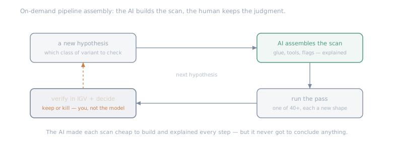
The AI made each scan cheap to build and explained every step. It never got to conclude anything — that stayed with the reads, and with me.

FASTQ, BAM, VCF: the three files

Before any of that made sense, I had to build a mental model of the three file formats the whole field runs on. If you come from data engineering, they map cleanly onto ideas you already have.

FASTQ is the raw data straight off the sequencer: millions of short reads — fragments of DNA a few hundred letters long — each with a per-base quality score saying how confident the machine is about each letter. It’s an unaligned, unordered pile. You can’t ask it “what’s at this position” yet, because nothing has a position. It’s the raw event log before you know what any of it means.

Aligning takes each read and finds where it belongs on the reference genome — the standard human assembly (GRCh38) everyone maps against. The result is a BAM: the same reads, now placed at genomic coordinates and sorted by position. Now you can point at a location and ask what’s there. Terminology that lives here: mapping quality (MAPQ, how confident the aligner is that a read belongs where it was put), and the reference itself, which is a consensus, not a truth — real people differ from it everywhere.

Variant calling compares the aligned reads to the reference and writes down every place this genome differs: a VCF, the Variant Call Format. Each row is one difference — its position, the reference letter, the alternate letter this person carries, the genotype (heterozygous, one copy, versus homozygous, both), and quality and depth numbers. The vocabulary: an SNV is a single-letter change, an indel is a small insertion or deletion, zygosity is whether one or both copies carry it.

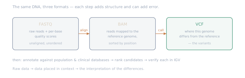
Raw data → data placed in context → the interpretation of the differences.

The mental model that helped most: each step adds structure and strips away rawness, and each step can also introduce error. A VCF is not “the truth about this genome.” It’s an interpretation produced by an aligner and a caller, each with assumptions, run over reads of varying quality. Treating the VCF as ground truth is exactly the ingestion-is-not-comprehension mistake I’ve watched wreck data pipelines at work. The data reached the system. That is not the same as the system being right.

Data quality is the hard part

We did whole-exome sequencing (WES): you sequence only the ~1–2% of the genome that codes for proteins — the exome. It’s far cheaper than doing the whole genome, and most known disease-causing variants sit in coding regions, so it’s a sensible first pass. The cost is everything it can’t see: deep-intronic and regulatory variants, most structural changes, repeat expansions, and anything in the 98% it never captured.

Within what WES does cover, the hard lesson was that a variant appearing in the VCF means very little on its own. Before I’d give any candidate a second look, I learned to check a specific set of attributes:

• Read depth (coverage) — how many reads cover the position. WES coverage is uneven; some exons capture poorly. A “variant” resting on 4 reads in a low-coverage patch might be noise. Below roughly 10–20×, I treated a call as a maybe, not a fact.
• Allele balance — for a heterozygous call you expect roughly half the reads to carry the variant. If it’s 15%, something is wrong: an artifact, a mapping error, or mosaicism. The number has to make genetic sense.
• Mapping quality — reads that could sit in several places (repetitive regions, gene families with near-identical copies) get low MAPQ. A variant built on low-MAPQ reads is often the aligner guessing.
• Strand bias — a real variant shows up on reads from both DNA strands. Support from only one strand is a classic artifact tell.
• Base quality, and PCR duplicates — the same original fragment amplified many times can look like independent depth while really being one observation counted five times; you de-duplicate before you trust the count. Indels near homopolymer runs and messy alignment regions throw false positives constantly.

The discipline that fell out of this was constant and manual: for essentially every candidate that survived the automated filters, I loaded the BAM into IGV, jumped to the exact coordinate, and looked at the reads by eye — the depth, the allele balance, the strands, whether it sat in a clean region or a swamp. I did this over and over, hundreds of times. Most candidates died right there on the pileup, and that death was the most valuable output of the whole exercise. The annotation surfaces a possibility; the pileup tells you whether it’s real. A ranked list is a list of hypotheses, not answers.

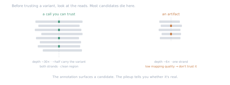
The annotation surfaces a candidate. The pileup tells you whether it’s real. (Illustrative — not real data.)

Rare in a database of Europeans is not rare in us

Here’s the part I think is genuinely underappreciated, and it’s a data problem more than a biology one.

Interpreting a variant leans heavily on population frequency — how often does this change appear in healthy people? A variant that’s vanishingly rare in the general population and lands in an important gene is interesting; one that a large fraction of healthy people carry is almost certainly just normal variation. The big reference databases exist to answer exactly this.

But those databases are built disproportionately from European-ancestry samples. South Asians are underrepresented. So a variant that is actually a common, benign polymorphism in South Asians can show up as “rare, possibly damaging” for the simple reason that not enough South Asians were ever sequenced to establish that it’s common and harmless. The rarity is an artifact of who’s in the reference set, not a property of the variant.

It cuts both ways. It manufactures false leads — benign-but-locally-common variants dressed up as suspicious — and it hides real ones, because population-specific pathogenic variants and founder effects in South Asian subpopulations are understudied and thinly characterized. For a family like mine, the practical consequence was a permanent asterisk on the word “rare”: rare in a database of mostly Europeans is not the same as rare in us, and every “rare, damaging” flag had to be read through that bias before it earned any excitement. It’s the oldest data lesson there is, wearing a genome: know whose data your reference was built from.

More resolution is exactly the thing that’s hardest to get

WES was the affordable door. But the honest truth is that higher-resolution sequencing would give a real search more to work with. Whole-genome sequencing (WGS) sees the parts WES never captures. Long-read sequencing — Nanopore, PacBio — resolves the structural variants, repeat expansions, and hard-to-map regions that short reads structurally struggle with, and it can phase variants (tell which copy a change sits on). More resolution means more chances to find the thing that a coarser method simply can’t see.

The catch, doing this from India, is that the higher-resolution option is exactly the one that’s hardest to get. Clinical-grade WGS and long-read are expensive; the labs offering them are few; turnaround is slow; sample logistics are real; and reanalysis — re-interpreting old data as the science improves — isn’t a routine, affordable service. Insurance rarely covers any of it, so each escalation is out of pocket. You end up in a quiet bind: the sequencing that might actually resolve the question is the sequencing you can least afford to keep redoing.

The tools a parent can actually reach

What genuinely surprised me is how much of the software is free and open, when not long ago it was strictly institutional. The ones I leaned on:

• IGV (Integrative Genomics Viewer) — load the BAM, jump to a position, and look at the reads. This was my verification workhorse, the tool that killed most false candidates. If you take one thing from this post: annotation proposes, IGV disposes.
• Franklin by Genoox — a free variant-interpretation platform that aggregates evidence and applies the standard ACMG classification framework, so you’re not eyeballing pathogenicity from scratch.
• OpenCRAVAT — an open annotation framework that runs many annotators over your variants at once: pathogenicity predictors, population frequencies, clinical databases, all in one pass.
• Galaxy — a web platform for running bioinformatics workflows without a local toolchain, which makes steps reproducible and shareable.

The barrier to doing this, it turns out, is no longer the software. It’s the data quality, the interpretation, the reference gaps, and the cost of better sequencing. The tools are the easy part now — which is its own version of the tutorial being the easy 5%.

We didn’t let the phenotype drive

The last discipline is the one I’m most sure about, and it’s the most transferable.

The obvious way to search is phenotype-first: take the clinical description — the symptoms — and look for genes known to cause them. The trouble is that the phenotype, as it reaches you, is noisy. It arrives through intake forms, doctors’ notes that recorded a parent’s offhand comment, early developmental observations that are subjective by nature, things reported under stress, a “maybe” written down as a “yes,” an ordinary toddler behavior over-interpreted in hindsight. Intake forms are full of red herrings — a noted symptom that was incidental, a detail that felt significant and wasn’t.

If you let that phenotype drive the search, you amplify whatever noise is in it. Filter your candidate genes by a symptom the child doesn’t really have, and you’ll either chase a gene that fits a phantom, or — worse — exclude the real gene because it doesn’t match a symptom that was mis-recorded in the first place. Phenotype-first search inherits every error in the phenotype.

So we deliberately didn’t. We anchored to two things: the genetic data itself — what the reads actually show, verified in the browser — and only the high-confidence phenotypes, the findings that were clearly and objectively documented and stable (a seizure disorder confirmed on its own terms, not “seemed a bit off one afternoon”). Everything softer than that was treated as a weak prior, a sanity check at most, never a filter. It’s the genomics version of a thing I believe about all data work: the human-supplied description of the problem is often the least reliable part of it, and when it conflicts with what the data plainly shows, you trust the data and re-examine the description.

None of this produced an answer — the essay this accompanies ends where it honestly has to, still unknown. But it produced something I do trust: a search that was honest about its own data quality, skeptical of its own reference set, and anchored to what the reads actually said instead of to what a form claimed. If the answer is ever in there, this is the only way I’d have believed it when I found it.